7.Moment tensor and "beach ball" calculation
10. Projection into the Line-Of-Sight
11. References
This tutorial is aimed at making the user familiar with the main modeling functionalities, by means of a complete modeling session of a seismic event, the Mw 6.6 earthquake occurred near the city of Bam (Iran) on December 26th, 2003. The tutorial starts with the Image Subsampling of a displacement map, then the coseismic displacement is modeled via Non-Linear Inversion and Linear Inversion, to retrieve the position of the fault and its slip distribution. The latter is then used to calculate the CFF Stress Transfer induced by the earthquake on the fault itself; finally, the retrieved model is used in a Forward Modeling to generate the raster maps of predicted displacement, projected into the Line-Of-Sight.
Though this tutorial gets through the main modeling features, it does not involve all the technical and scientific modeling aspects. In most cases, only one of the possible processing configurations is presented: we strongly suggest the user to refer to the linked help pages for a complete description of all the available options.
We remark that modeling is, in general, a non-unique problem: different solutions can lead to comparable results, equally able to reproduce the observed data. Only the experience and an incisive data analysis can lead to realistic solutions.
Tips and Notes are provided to improve the modeling strategy and/or highlight further software functionalities.
This tutorial is based on the displacement map generated with a pair of SAR images acquired by the Envisat satellite from the European Space Agency. This map has been obtained with an interferometric processing carried out with the SARscape interferometric module; the images have been acquired on December 3rd, 2003 and February 11th, 2004 and have a spatial baseline of about 4 m. In this tutorial the displacement is modeled with a single fault with distributed slip.
Refer to the cited literature (Wang et al., 2004; Funning et al, 2005) for a review of the event.
REFER TO YOUR LOCAL DISTRIBUTOR TO GET THE DATA FOR THIS TUTORIAL.
To run the tutorial, you need the following files:
•Bam_envisat_dsc_disp: displacement map (m) obtained from a descending Envisat image pair;
•Bam_envisat_dsc_ALOS: map of the Line-Of-Sight azimuth angle (deg);
•Bam_envisat_dsc_ILOS: map of the Line-Of-Sight incident angle (deg);
•Bam_SRTM_dem: SRTM digital elevation model with 90 m resolution;
•Bam_project_backup.xml: XML Project File (see next paragraph);
•Subsampling_areas.shp: shapefile containing the areas to sample the displacement map.
All the images are in a UTM-WGS84, Zone 40 North, projection.
The main modeling panels requires the setting of an XML Project File. This file allows to save the input configuration of any processing for a quick restore in any moment. Most of the processing outputs are stored in the XML Project File as well, allowing an efficient project portability.
In this tutorial, an XML Project File created from scratch and named Bam_project.xml will be used. Though a project file with all the sections already set is provided with the tutorial data (Bam_project_backup.xml), we suggest the use of a new one to get confident with its use.
Since modeling is predomintaly carried out with vector data, Image Subsampling is a mandatory task to create a vector dataset of values sampled from the InSAR displacement maps.This can be due in two ways: by sampling the image over regularly spaced points in manually defined areas (mesh from vector file) or with the Quadtree algorithm. In this tutorial we use the first approach, which needs the definition of the areas and their sampling resolution by means of a shapefile. This file is provided with the input data (Subsampling_areas.shp) where two areas with density 500 m and 2000 m, close and far from the fault, respectively, are already set (Fig. 1).
| Tip | You can define different subsampling areas and resolutions, by editing the shapefile or creating a new one (see mesh from vector file); in this way a different dataset to model is obtained and results may differ from this tutorial. |
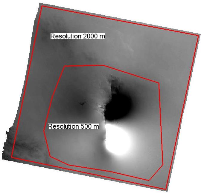
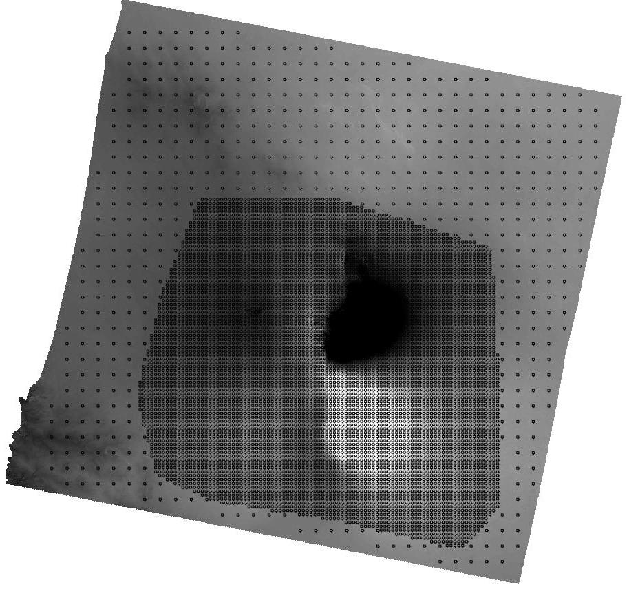
Figure 1. Sampling areas with resolution values (left) and resulting points (right)
Once the file with the sampling areas is available:
1.Open the Image Subsampling panel;
2.Set the following files:
•“Subsampling Image”: Bam_envisat_dsc_disp
•“Azimuth LOS image”: Bam_envisat_dsc_ALOS
•“Incidence LOS image”: Bam_envisat_dsc_ILOS
•“DEM”: Bam_SRTM_dem
3.Set Mesh from vector file as “Subsampling method”
4.Set in “Vector File” the Subsampling_areas.shp file (or a newly created one)
5.Set in “Output Shapefile” the Bam_sampled_points.shp name
6.Click “Start” and wait for the “END” message.
By using the Subsampling_areas.shp as it is provided with the tutorial data, the Bam_sampled_points.shp will contain 7448 points (Fig. 2) with the related attributes. This shapefile of points represents, in the modeling tools, an InSAR dataset.
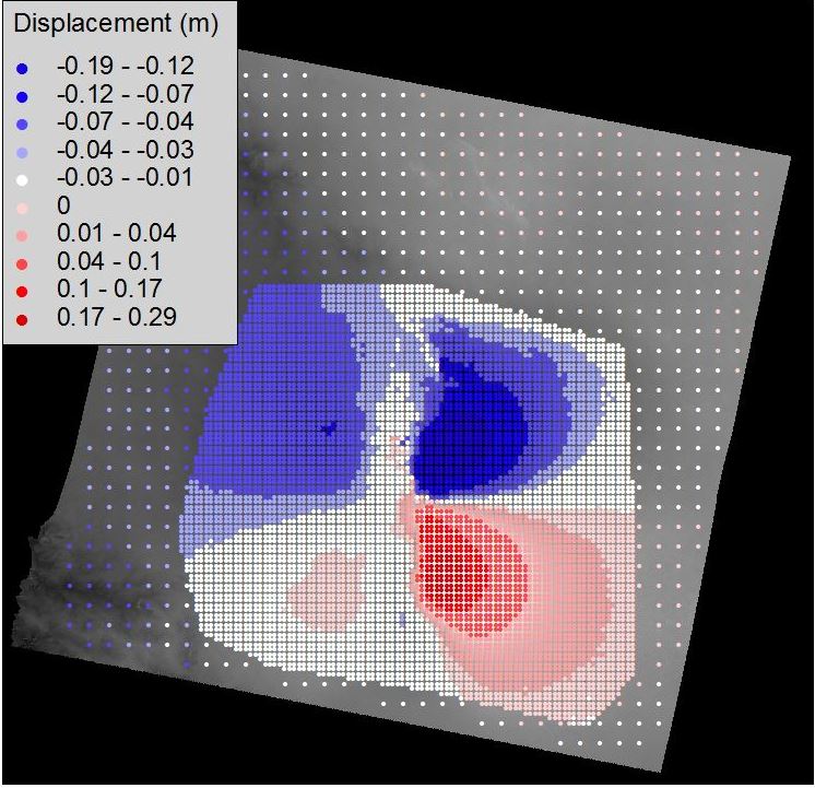
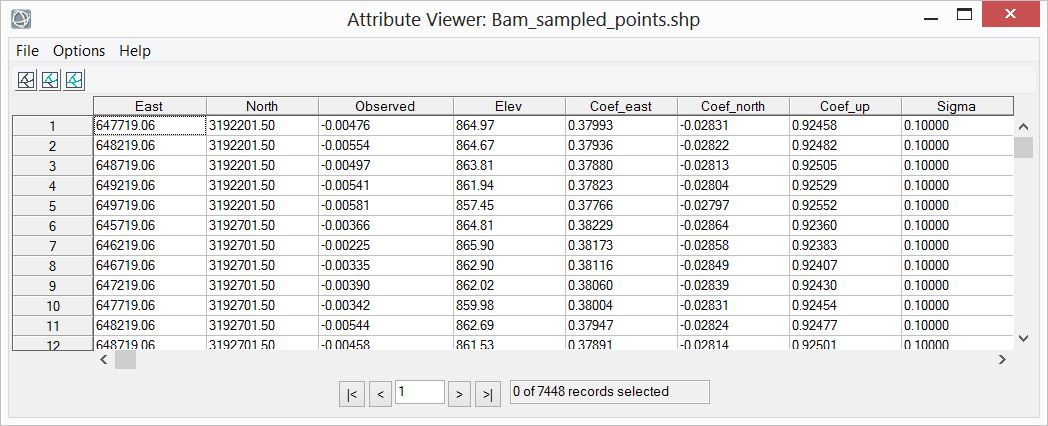
Figure 2. Subsampled points and relative attributes
| Note | In addition to the known shapefile components (.shp, .dbf, .shx and .prj files) a further file is created (Bam_sampled_points.shp.xml) with ancillary information required by the inversion. This file is generated only when subsampling is carried out over a displacement map created with SARscape; in the other cases, its content must be manually set through the interface. |
With the Non-Linear Inversion we want to reproduce the observed displacement by means of a geophysical source, assuming that nothing is known about the source and all its parameters must be inferred from the InSAR dataset just created. In this tutorial we model the data with a single fault (see Elastic Dislocation), but we invert also a further parameter, accounting for a possible offset that could affect the data; this is advisable when the reference point in the interferogram could have been set in a deforming area.
In the Non-Linear Inversion the use of the XML Project File is mandatory and must be set:
1.Open the "Non-Linear and Linear Inversion” panel;
2.Select the “Non-Linear” tab;
3.Set the “XML Project File” to Bam_project.xml.
Dataset setting
The InSAR dataset created with the displacement map subsampling is added as follows:
1.Click on the “Add…” button in the “Dataset(s)” list and select the Bam_sampled_points.shp;
2.Open the Parameter setting panel through the “Edit…” button;
3.Flag the “Invert for orbital surface” (default option);
4.Set 0 as “Polynomial degree”;
5.Click on “Commit”.
By setting 0 as polynomial degree, you let the inversion to assess also a possible offset that may affect the data.
Source setting
In this tutorial we assume that all the source parameters are unknown; however, we must set, for each parameters, a range of allowed values between a minimum and a maximum. Since the Elastic Dislocation source is characterized by an high number of parameters, we developed a specific tool to initialize the source based on the Global Centroid Moment Tensor on-line catalogue. This tool only needs the CMT event identifier, which can be preliminarily retrieved as follows:
1.Open the http://www.globalcmt.org/CMTsearch.html site;
2.Set the following parameterse:
·Starting Date - Year: 2003
·Starting Date - Month: 12
·Starting Date - Day: 26
·Ending Date - Number of days: 1
·Moment magnitude range with 6 <= Mw <= 7
3.Click on “Done”;
4.Two events should fit this constraints: we will use the identifier of the “SOUTHERN IRAN” event (122603B).
Once the CMT event identifier is known, you can initialize the source to invert:
1.In the Non-Linear Inversion panel, click on the “New…” button from the “Source(s)” list;
2.Select Elastic dislocation (Okada) from the pull down menu;
3.Click on the "Initialize from CMT solution…" button to open the Initialize Values from CMT Catalogue panel;
4.Set the event identifier (122603B) in the “Insert the CMT identifier” field and click the “Search” button (it could take a while to get the result);
5.From the pull down menu select “Plane 1” then click “Commit”;
6.Set “Bam_fault” as “Source name”, then click “Commit” to return to the main panel;
7.Click on the “Start” button to run the inversion;
8.Click “Yes” to the “XML Project File updated” dialog box;
9.Wait until the “END” message (it could take few minutes);
10.Click “No” to the “Focal Mechanism” dialog box
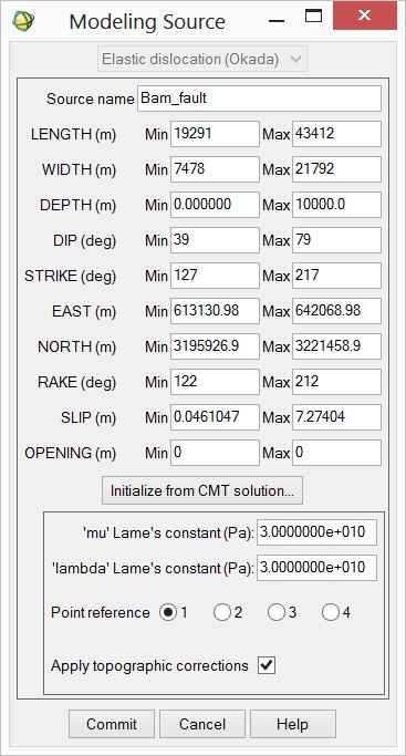
Figure 3. Source parameters automatically initialized with the CMT solution
| Tip | The CMT catalogue provides two alternative solutions, corresponding to two possible nodal planes: the real slipped plane and the auxiliary one, which is only a mathematical solution. In the case of Bam, the displacement pattern clearly shows that the fault plane is nearly North-South oriented, which corresponds to the “Plane 1” solution in the Initialize Values from CMT Catalogue panel. |
| Note | When the XML Project File file is updated, the “NLInput” and ”NLOptions” sections are created under the “ModelingRoot”-”NonLinearInversion” XML section. If they already exist from a previous processing, they are overwritten. In order to maintain the alignment between input parameters and output models, when the “NLInput” and ”NLOptions” sections are updated, the “NLOutput” section, if existing from a previous processing, is canceled. |
When the Non-Linear Inversion ends, the Bam_project.xml file is updated with the results: inverted model parameters, InSAR data offset, RMS of the residuals between observed and modeled data, geodetic moment, moment magnitude, etc… All the information are written in the “ModelingRoot”-”NonLinearInversion”-”NLOutput” section.
| Note | the Non-Linear Inversion algorithm is based on multiple restarts: every starting configuration is randomly picked within the allowed ranges to avoid, as far as possible, to trap the cost function into local minima. This aleatory component can lead to different results with repeated runs. |
| Tip | We strongly suggest to run the Non-Linear inversion several times and inspect every time the inferred source, in order to understand the reliability and the stability of a result. |
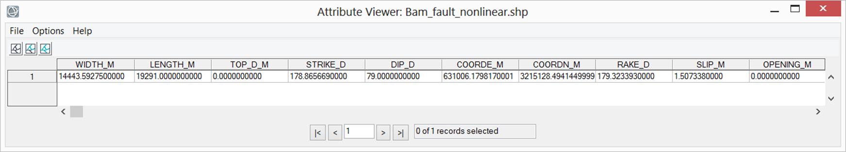
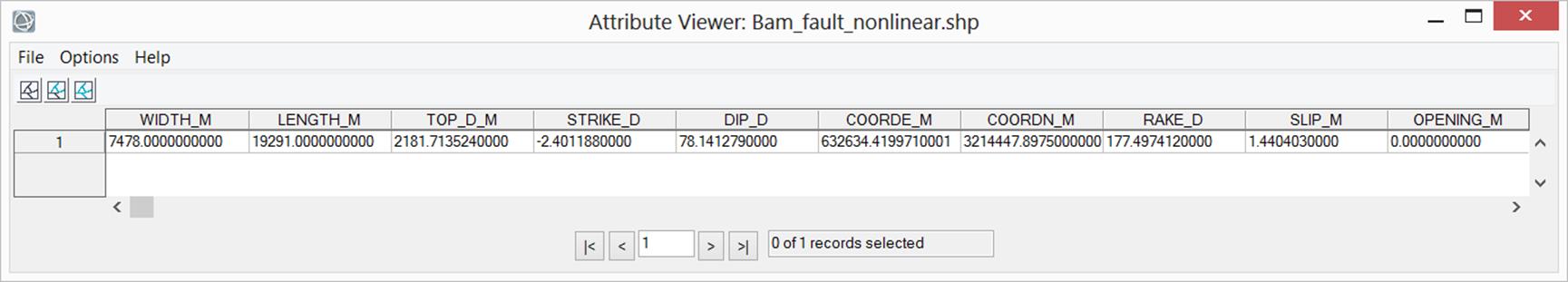
Here we show the result obtained with the source initialized as in Fig. 3. If the flags “Generate output shapefile” in the Inversion Settings (accessible through the “Inversion settings…” button in the inversion panel) are set, the following files have also been created:
•Bam_fault_nonlinear.shp, with the best fit source and its parameters as attributes;
•Bam_sampled_points_nonlinear.shp, containing the observed and modeled data (see the output attributes after the inversion for the InSAR dataset).
From the XML Project File |
|
Overall residual RMS |
0.028 m |
Geodetic Moment |
1.26 ∙1019 N∙m |
Moment Magnitude |
6.7 |
Data offset |
0.014 m |
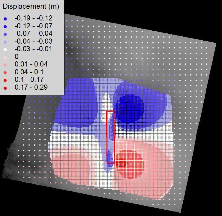
Figure 4. Modeled points, fault parameters and other general parameters after the Non-Linear Inversion automatically initialized with the CMT values.
The results of Fig. 4 show that the source automatic initialization with CMT values has already led to reasonable results. However further improvements of the Non-Linear Inversion are still possible.
| Tip | When a parameter reaches the upper or the lower limit of the allowed range after the inversion, the range should be modified to let the algorithm explore other possible values. A good result is achieved when all the parameters fall within the specified range without assuming any limit value. |
| Tip | When a parameter is already known, you can fix it by setting the minimum and maximum to the known value. |
In Fig. 4 the "Dip" reached the upper limit (79°), and this indicates that higher values could be preferred. In fact, the "Strike" and "Dip" ranges only allow to explore westward dipping faults, while the deformation pattern suggests an eastward dipping plane (see Fig. 1). Therefore we run again the Non-Linear Inversion with modified “Strike” and “Dip” ranges, as shown in Fig. 5 (see the Elastic Dislocation source for "Strike" and "Dip" angle conventions). To set the new ranges click on the “Edit…” button under on the “Source(s)” list.
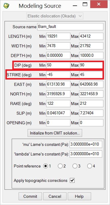
Figure 5. Modified ranges (in red) for the second inversion with a eastward dipping source
After editing the ranges, run again the Non-Linear Inversion and check that all the parameters now fall within the ranges. You can also navigate through the “NLOutput” section of the Bam_project.xml file to verify that the RMS of the residuals is slightly lower than before, showing that this second solution better reproduces the observed data.
From the XML Project File |
|
Overall residual RMS |
0.026 m |
Geodetic Moment |
0.62 ∙1019 N∙m |
Moment Magnitude |
6.5 |
Data offset |
0.017 m |
Figure 6. Modeled points, fault parameters and other general parameters after the Non-Linear Inversion with revised ranges for "Strike" and "Dip".
| Note | Different solutions can fit almost equally the observed data, as visible by comparing the RMS of the residuals between observed and modeled data of Fig. 4 and Fig. 6. The RMS is nearly the same, in spite of the different sources. Only external information and the experience help in understanding whether a solution is reliable or not. |
With the Non-Linear Inversion a mean source with a mean and unique slip value of 1.44 m has been inferred (Fig. 6). With the Linear Inversion we retrieve a more realistic slip distribution over the fault plane by means of a Elastic dislocation model. Before the inversion parameter setting, the XML Project File must be specified:
1.Open the “Non-Linear and Linear Inversion” panel;
2.Select the “Linear” tab;
3.Set the “XML Project File” to Bam_project.xml.
| Note | In this tutorial, we collect all the tasks in the same XML Project File. However, tasks are independent and can be stored separately in different project files. |
Dataset setting
The InSAR dataset to invert is loaded as in the Non-Linear Inversion (just make sure you switched to the “Linear Inversion” tab in the panel):
1.Click on the “Add…” button in the “Dataset(s)” list and select the Bam_sampled_points.shp;
2.Open the Parameter setting panel through the “Edit…” button;
3.Flag the “Invert for orbital surface” (default option);
4.Set 0 as “Polynomial degree”;
5.Click on “Commit”.
Source setting
The starting point of the Linear Inversion, in this tutorial, is the source calculated through the Non-Linear Inversion: instead of creating a new source from scratch with the “New…” button, we load the Non-Linear Inversion results. This can be done in two ways: loading the Bam_fault_nonlinear.shp (created after the inversion) through the “Add from file…” button or retrieving the plane parameters with the “Load from XML…” button, which allow to explore the content of any XML Project File.
| Note | The “Add from XML…” button allows to access any XML Project File, to inspect and retrieve any stored source (input/output of Non-Linear Inversion, Linear Inversion, CFF Stress Transfer, Forward Modeling). Here, we access the same Bam_project.xml file to get the output of the Non-Linear Inversion. |
To extract the source from the XML Project File:
1.Click on the “Load from XML…” button under the “Source(s)” list;
2.Select the Bam_project.xml file;
3.In the XML section, select “Non-Linear Inversion - Output”;
4.Select, from the “Bam_fault [Elastic dislocastion (Okada)]” item;
5.Click “Commit”.
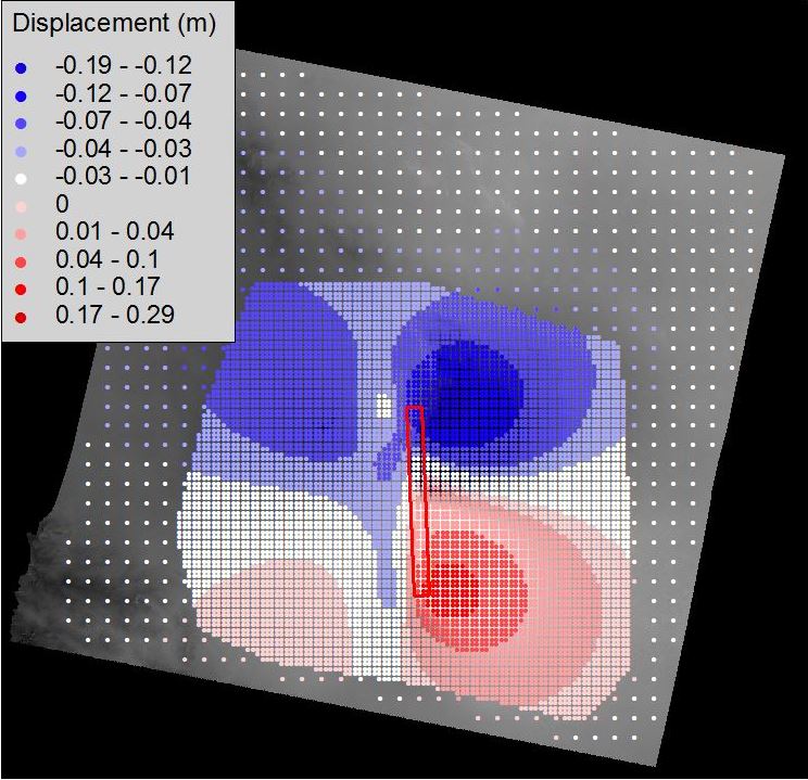
| Tip | Since the slip retrieved through Non-Linear Inversion is a mean value of the real one, it is always convenient to extend the fault dimensions to include the whole slipped area, letting the slip to vanish at the fault limits (Fig. 7). |
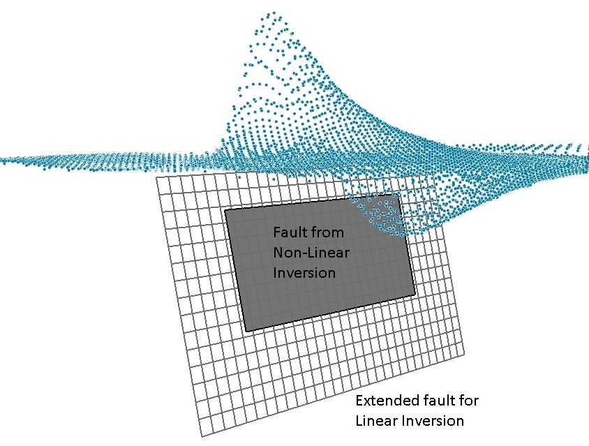
Figure 7. Fault from Non-Linear Inversion (gray rectangle) extended and subdivided into 30x15 patches; blue points represent the observed displacement in the Line-Of-Sight.
The source retrieved from the Non-Linear Inversion is added to the “Source(s)” list with the flag “*** CHECK PARAMETERS ***”, notifying that more information must be provided before running the inversion. To complete the source setup and change the source dimension:
1.Select the source in the “Source(s)” list and click the “Edit…” button;
2.Change the “Point reference” to 4;
3.Set the “Length (m)” field to “30000.”;
4.Set the “Width (m)” field to “15000.”;
5.Set the “Depth (m)” field to “0.”;
6.Set “Fixed rake” as Inversion Type;
7.Set the “PATCHES ALONG STRIKE” field to “30” and “PATCHES ALONG DIP” field to “15”;
8.Set the “Damping value” to 0.05
9.Only for ENVI 5.0 or higher, click the “Draw Source in ENVI 5.x” button to see the source in the ENVI view (a reference layer must be already present);
10.Click the “Commit” button;
11.Click on "Start" to run the inversion;
12.Answer “No” to the “Focal Mechanism” dialog box after the inversion ends.
| Note | By switching the Point Reference to 4 (see the Point Reference in the Elastic dislocation source), the source length, width and depth can be changed without affecting the East and North coordinates, that are referred to the unchanged fault trace. |
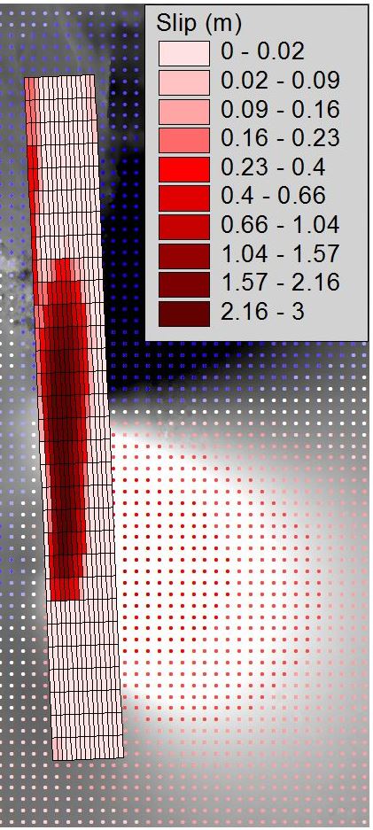
In the Linear Inversion we extended the initial fault to a 30x15 km source, subdivided into patches of 1 km. After clicking on the “Start” button, the Bam_project.xml file is updated: the ”LinInput” and ”LinOptions” sections in “ModelingRoot”-”LinearInversion” are immediately created (or updated), while the "LinOutput" section is added at the processing end. The results of the Linear Inversion are shown in Fig. 8.
From the XML Project File |
|
Overall residual RMS |
0.012 m |
Geodetic Moment |
0.53 ∙1019 N∙m |
Moment Magnitude |
6.4 |
Data offset |
0.017 m |
Figure 8. Modeled points, slip distribution and other parameters after Linear Inversion
| Tip | The slip distribution strongly depends on the Damping Value: a low damping leads to scattered slip values while high values to an over-smoothed solution. The best value can be obtained only with a trial-and-error approach. Unless you want a complete damping vs. RMS curve, we suggest a divide-and-conquer algorithm: start from a low value, then move to a high value, then test a value in between, and so on… checking at every step the result. This is quite fast, if the output shapefile is loaded into a GIS: since the output shapefile, at every step, is overwritten, you just need to refresh the view to check the result for every new damping value. |
If the flags “Generate output shapfile” in the Inversion Settings (accessible through the “Inversion settings…” button in the inversion panel) are set, the following files have been created:
•Bam_fault_linear.shp: containing the best fit source and its parameters;
•Bam_sampled_points_linear.shp: containing the observed and modeled data (see the output attributes after the inversion for the InSAR dataset)
7. Moment Tensor and “beach ball” calculation
The Calculate and Draw Focal Mechanism panel can be used to calculate the seismic moment, to moment tensor and to draw the beach ball of the focal mechanism. This can be accomplished with a new source created from scratch or loading an existing source from a shapefile or an XML Project File. In this tutorial, we load the results of the Linear Inversion from the Bam_project.xml file:
1.Open the Calculate and Draw Focal Mechanism panel;
2.Click on the “Add from XML…” button;
3.Select the Bam_project.xml file;
4.Form the “XML section” pull down menu, select “Linear Inversion – Output”;
5.Select in the source list the “Bam_fault [Fault patches(Okada)]” item and click “Commit”;
6.In the main panel, select the source just loaded and click “Start” (Fig. 9).
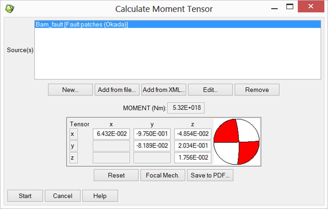
Figure 9. Moment tensor and focal mechanism for the modeled source of the Bam earthquake
| Tip | You can test, for instance, the effect of changing the shear modulus μ just editing the source through the “Edit…” button and setting a different value in the “’mu’ Lame’s constant” field. |
This tool can be used to calculate the stress change induced by one or more sources onto other sources acting as receivers. In the case of Bam, where only one source is involved, we calculate the stress change induced by the fault on the slipped plane itself.
| Tip | The self-induced stress change can be used, for instance, to check whether the aftershock distribution is coherent with the highest loaded areas. |
This task requires the setting of the XML Project File:
1.Open the CFF Stress Transfer panel;
2.Set the “XML Project File” to Bam_project.xml.
The input and receiver sources are retrieved, as in previous tasks, from the Bam_project.xml file itself:
1.Click on the “Add from XML…” button under the “INPUT SOURCE(S)” list;
2.Select the Bam_project.xml file;
3.From the “XML section” pull down menu, select “Linear Inversion – Output”;
4.Select in the source list the Bam fault item and click “Commit”;
5.Click on the “Add from XML…” button under the “RECEIVER SOURCE(S)” list;
6.Repeat the steps from 2 to 4;
7.Set the flag "Automatically create output Shapefiles";
8.Click on the “Start” button in the main panel and wait for the “END” message.
After the processing, the output source, i.e. the receiver with the CFF values, can be loaded into a GIS, as in Fig. 10.
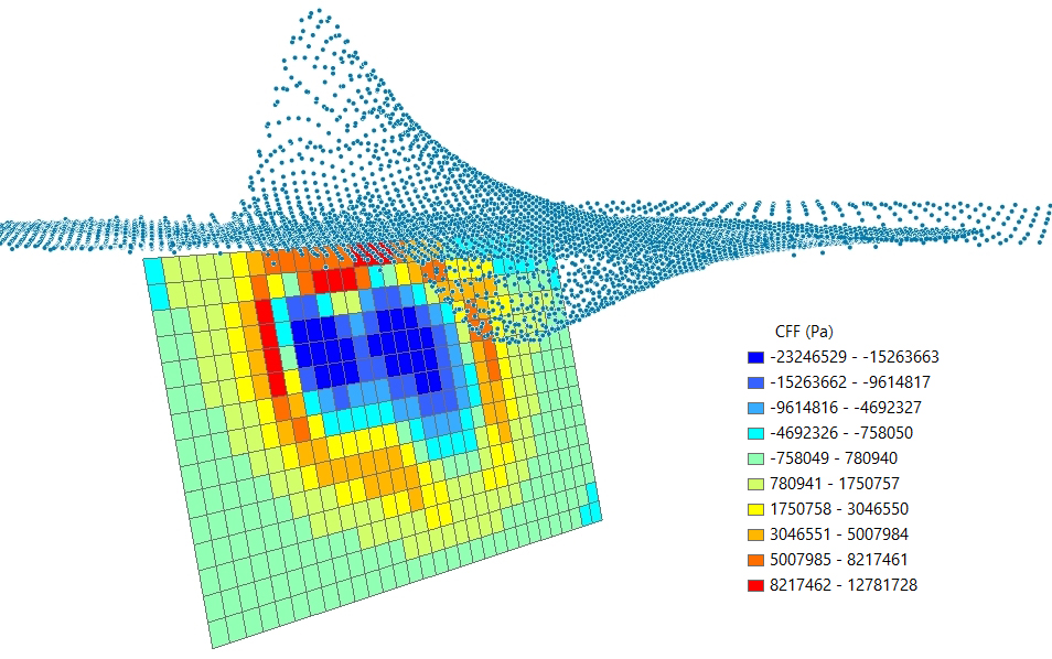
Figure 10. Stress change induced by the slip of Fig. 8, over the Bam fault itself.
In this step, we use the source obtained via Linear Inversion to calculate the surface displacement in the East, North and Up directions. Forward Modeling can be carried out over a set of points, stored in a shapefile, or creating three raster files containing the East, North and Up components. In this tutorial we create a raster output, using the Bam_envisat_dsc_disp (the original displacement map from the interferometric processing) as reference to set the output extent and resolution. The latter is reduced from 25 m to 250 m to speed up the processing.
| Tip | For big earthquakes, the USGS website makes available a slip distribution obtained through the inversion of seismic waveforms. The tool Import USGS Slip Distribution can be used to generate the source in a shapefile form; the source can be then loaded with the "Add from file..." button in the Forward Modeling source list to generate the surface displacement maps. |
This task requires the setting of the XML Project File:
1.Open the Forward Modeling panel;
2.Set the “XML Project File” to Bam_project.xml.
| Note | We remark that with in this release, any modeling processing must be carried out in a projected cartographic system; in the case of Bam, data are in the UTM-WGS84, Zone 40 North, projection. |
To create the raster maps of the surface displacement:
1.Click on the “Add from XML…” button under the “INPUT SOURCE(S)” list;
2.Select the Bam_project.xml file;
3.From the “XML section” pull down menu, select “Linear Inversion – Output”;
4.Select in the source list the “Bam_fault [Fault patches(Okada)]” item and click “Commit”;
5.In the “Forward Model Output” pull down menu, select “Raster”;
6.Click on “Get from image…” and select the Bam_envisat_dsc_disp file;
7.Change, if necessary, the “Output File” name and the path automatically created;
8.Check on the “Set raster info…” button;
9.Change to 250 the “Cell size”;
10.Click on the “Cartographic System” button and set the following parameters:
•“State”: UTM-GLOBAL
•“Hemisphere”: NORTH
•“Projection”: UTM
•“Zone”: 40
•“Ellipsoid”: WGS84
11.Click on “Commit” to close the “Set cartographic system” panel;
12.Click on “Commit” to close the “Raster Parameters”;
13.Click on “Start” and wait for the “END” message.
Unless you changed the output name, automatically generated, the processing will create the following files (Fig. 11):
•Bam_envisat_dsc_disp_forward_east: with the displacement East component;
•Bam_envisat_dsc_disp_forward_north: with the displacement North component;
•Bam_envisat_dsc_disp_forward_up: with the displacement Up component.
After Forward Modeling, the Bam_project.xml file is automatically updated with the section “ModelingRoot”-“ForwardModeling”. You can navigate through the XML tags to inspect its content.
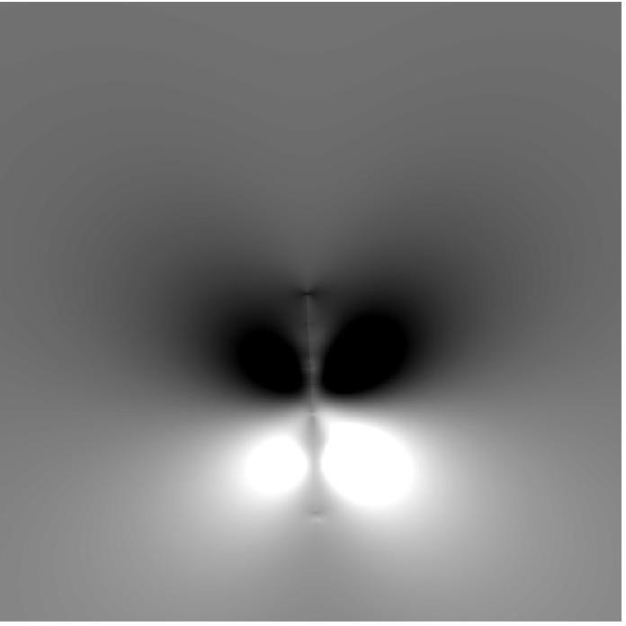
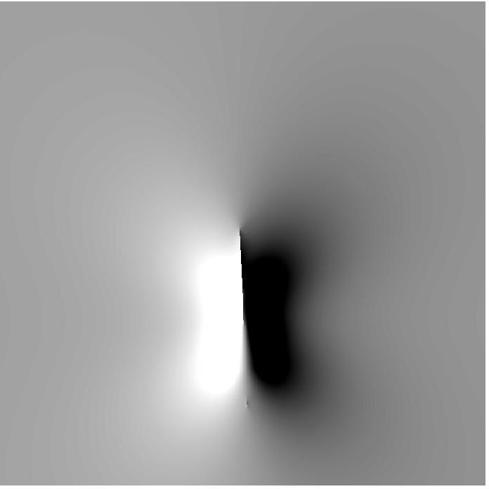
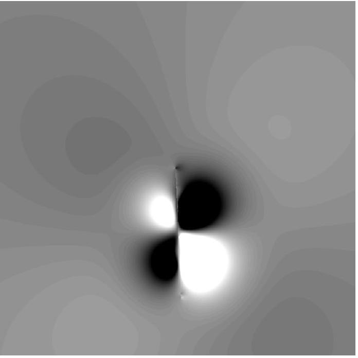
Figure 11. East, North and Up components of the displacement generated by the slip distribution retrieved via Linear Inversion.
| Note | The displacement measurement unit is always coherent with the input source: if the slip is provided in meters, the output displacement will be in meters. |
10. Projection into the Line-Of-Sight
In the last step, the three maps resulting from Forward Modeling are combined together and projected into the direction of a specific Line-Of-Sight. This panel just needs the three raster maps and the ALOS (Azimuth Line-Of-Sight) and the ILOS (Incidence Line-Of-Sight) images.
| Note | The group of the East/North/Up displacement maps and the ALOS/ILOS pair have in general different extents and resolutions; extent and resolution of the output raster can be independently set according to any of the two groups. |
| Tip | When several LOSs are available (perhaps Ascending and Descending) Forward Modeling can be done just once to create the East/North/Up displacement maps; then they can be projected into as many LOSs as available. |
To run the LOS projection:
1.Open the Project raster to LOS panel;
2.Set the following files:
•“East component”: Bam_envisat_dsc_disp_forward_east
•“North component”: Bam_envisat_dsc_disp_forward_north
•“Up component”: Bam_envisat_dsc_disp_forward_up
•“Azimuth LOS image”: Bam_envisat_dsc_ALOS
•“Incidence LOS image”: Bam_envisat_dsc_ILOS
3.Set the “Output image” to Bam_envisat_dsc_disp_forward_los;
4.Set the “Raster extent” to “Same as the ALOS/ILOS components”;
5.Set the “Raster resolution” to “Same as the ALOS/ILOS components”;
6.Click on the “Start” button and wait for the “END” message.
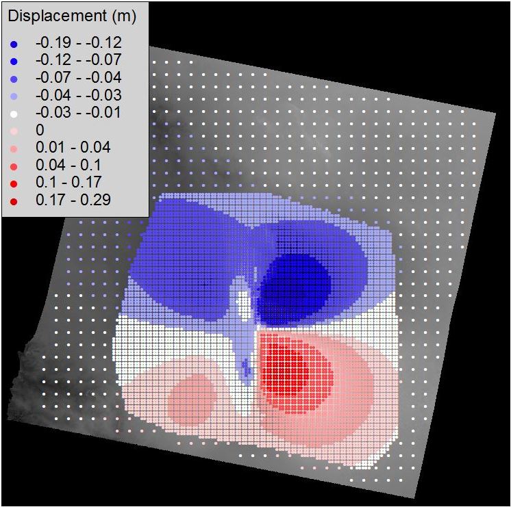
After that, you can compare the Forward Modeling results projected into the LOS with the original displacement map, as in Fig. 12.
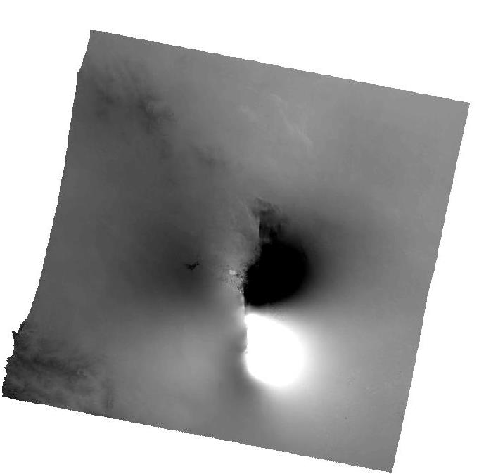
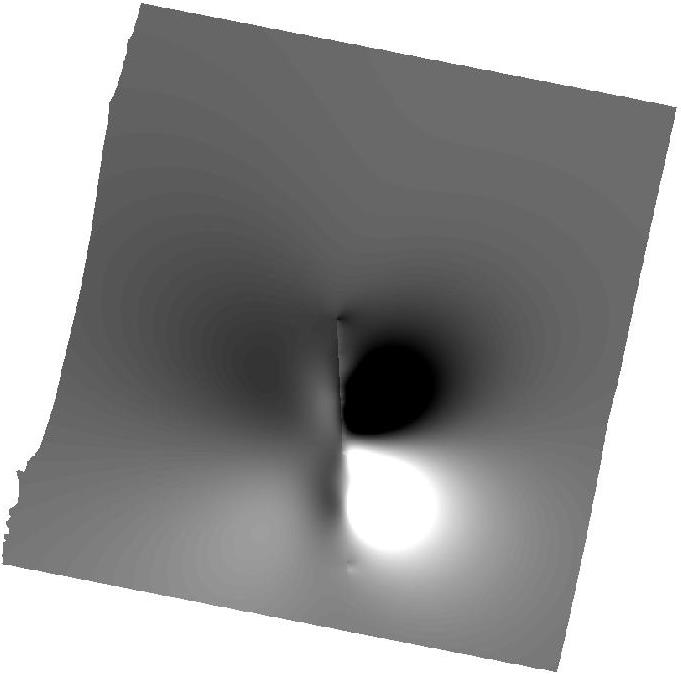
Figure 12. Comparison between the observed (left) and the modelled (right) displacement maps in the Line-Of-Sight
| Note | To make a fair comparison between the observed and modeled displacement maps, it must be taken into account that in the inversion an orbital surface could have been assessed. |
In this case, we calculated in the Linear Inversion an offset of 0.017 m (see Fig. 8); this value must be added to the modeled displacement of Fig. 12 (right) to obtain the complete modeled displacement.
Funning, G.J., B. Parsons, T.J. Wright, J.A. Jackson and Fielding, E. J. (2005), Surface displacements and source parameters of the 2003 Bam (Iran) earthquake from Envisat advanced synthetic aperture radar imagery, J. Geophys. Res., 110, B09406, doi:10.1029/2004JB003338.
Wang, R., Xia, Y., Grosser, H., Wetzel, H.-U., Kaufmann, H. and Zschau, J. (2004), The 2003 Bam (SE Iran) earthquake: precise source parameters from satellite radar interferometr, Geophy. J. Int., 159: 917–922. doi: 10.1111/j.1365-246X.2004.02476.x
© sarmap, January 2013