Purpose

This panel is used to set the parameters for the Elastic dislocation source, according to the formulation of Okada [1985].

Technical note

This analytical source is used to predict the surface displacement induced by a rectangular dislocation in homogeneous and elastic half-space [Okada 1985]. It is adopted in the modeling of earthquakes, sills, dike intrusions, etc. Model parameters required to describe its geometry and kinematic are shown in Fig. 1.

The Okada source is implemented in two forms:

- single source with uniform slip/opening, as shown in Fig. 1;

- planar array of sources, with distributed slip/opening, as shown in Fig. 2.

The distributed source is generally obtained by dividing a uniform slip sources into a number of elements (patches) along the strike and dip directions. Typically, within an inversion process, a Non-Linear Inversion is used to obtain all the parameters of the uniform slip source; the resulting source is then subdivided into elements, whose slip/opening values are retrieved by Linear Inversion. This allows to simulate a more realistic source model, as described in the Modeling Tutorial 1.

The source setup panel has a different appearance, according to the processing phase (Non-Linear Inversion, Linear Inversion, Forward Modeling, CFF Stress Transfer, Calculate and Draw Focal Mechanism). Moreover, only for the Non-Linear Inversion, the user must not set a single value for parameters of Fig. 1, but a range (minimum/maximum) of allowed values to search for the best-fit solution.

Elastic dislocation source

Figure 1. Source parameters of the Elastic dislocation (Okada)

Distributed elastic dislocation source

Figure 2. Source parameters for a distributed Elastic Dislocation (Okada)

About the Strike, Dip angle convention. The Strike angle is counted clockwise from the North to the trace direction; of the two possible trace directions, it is considered the one such that the source is dipping at right, as in Fig.1. The Dip angle has values ranging from 0° (horizontal source) to 90° (vertical source) and values out of this range are considered wrong: sources dipping at left (dip > 90°) must be instead represented as dipping at right with the opposite strike direction. For example, a source with Strike 30° and Dip 100° must be represented with Strike 210° (30°+π) and Dip 80°.

About the Rake convention. The Rake describes the shear direction, considering the displacement of the overlaying surface relative to the underlying surface; in Tectonics, the hanging wall with respect to the footwall. The Rake angle varies from -180° to 180° and is calculated as shown Fig. 3. According to the seismological terminology, the earthquake mechanism is left-lateral for rake 0°, thrust or inverse for rake 90°, direct or normal for rake -90° and right lateral for rake 180° or -180°. Rake values are "wrapped": negative values or greater than 360 are converted to 0-360 (for example: 200° is equal to -160°).

Rake angle convention

Figure 3. Convention on the Rake angle

About the reference point. Four alternative ways are provided to describe the source position and depth (see Fig. 4):

1 - East and North coordinates of the source center, vertically projected on the surface; depth, in meter, is calculated between source upper edge and the surface (positive downward);

2 - East and North are referred to the source upper-left corner; depth is the same as 1;

3 - East and North are referred to the center of the source upper edge; depth is the same as 1;

4 - East and North are referred to the source (fault) trace center; depth is the upper edge distance from the trace. This notation can not be used when Dip = 0.

Though these alternatives are absolutely equivalent, sometimes it is more convenient to adopt one in particular. For example, some earthquakes are generated by a fault with a known trace, either from literature or because the rupture reached the surface; in this situation, the notation 4 is particularly useful, because changing dip and depth does not affect the reference point.

okada_notations

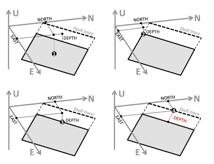
Figure 4. Reference point used to define the source position and depth

About topographic corrections. Analytical equations provide the displacement at the surface of the elastic half-space, considered as zero-level. For areas with strong topography, the depth from the flat half-space can significantly differs from that of the real surface. A strategy adopted to account for this difference is to sum the source depth and the point elevation above the zero level in the displacement calculation (Fig. 5). This can be done when the topographic elevation is available for the modeling dataset (see the Image Subsampling tool) by setting the "Compensate for Topography" flag.

topo_corrections

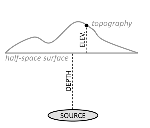
Figure 5. Source depth and point elevation composition in modeling

Input Parameter(s)

Length

Source length, in meters.

Width

Source width, in meters.

Dip

Angle between the source and the surface, in degrees (see the Technical Note and Fig. 1).

Strike

Angle between the source trace and the North, in degrees (see the Technical Note and Fig. 1).

Rake:

Dislocation angle, in degrees (see the Technical Note and Fig. 3).

Slip:

shear dislocation over the plane, in meters.

Opening:

Tensile dislocation perpendicular to the source, in meters, describing a source opening or closure.

Depth

Source depth, positive downward, in meters; read the Technical Note to see how it is calculated according to the Reference Point (Fig. 4) .

East, North

Coordinates of the source reference point (see the Technical Note and Fig. 4), UTM or Lat/Lon.

Reference Point

Point used to define the source position (see the Technical Note and Fig. 4):

1.Fault center - Vertical top edge

2.Upper left corner - Vertical top edge

3.Top edge center - Vertical top edge

4.Fault trace center - Along dip top edge

Linear inversion input options

Fixed Source

By setting this flag, no parameters are retrieved by inversion; its contribution is removed from signal before modeling (it's particularly useful for overlapping events)

Variable Size Patches

This flag allow the automatic retrieval of the "full resolution" fault subdivision according to Atzori and Antonioli [2011].

Patches along strike

Number of subdivisions along strike (leave 1 if checked 'Variable Size Patches').

Patches along dip

Number of subdivisions along dip (leave 1 if checked 'Variable Size Patches').

Linear inversion types:

Distributed and positive slip with fixed rake

Non-negativity constraint is applied: only positive (or zero) slip values are returned, with a fixed rake direction

Distributed slip with fixed rake

Positive and negative slip can be returned, with a fixed direction

Distributed slip with variable and bounded rake

Positive (or zero) slip values are returned, in a range centered about the given rake.

This choice allows to set the Rake range width.

Distributed slip with free rake

Slip values and rake directions are both retrieved by inversion.

Distributed Opening

Only opening values are allowed from the inversion.

Distributed Closure

Only the closure values are allowed from by inversion.

Distributed Opening/Closure

Positive (opening) and negative (closure) tensile components are retrieved by inversion.

Ancillary Parameters

'mu' and 'lambda' Lame's constant

Lame's constant of the elastic medium, in Pascal (see Preferences).

Compensate for topography

The processing is carried out accounting for the local topography (see the Technical Note and Fig. 5).

Coordinate System

Coordinate system of the source; if not set, it can be defined with the 'Set...' button

Specific Function(s)

Draw Source in ENVI 5.x

Draw the source in the ENVI 5.x view.

General Functions

Commit

End the source parameter editing.

Cancel

The window will be closed.

Help

Specific help document section.

References

Atzori, S. and A. Antonioli (2011), Optimal fault resolution in geodetic inversion of coseismic data, Geoph. J. Int., 185 (1), 529-538.

Okada, Y. (1985), Surface deformation due to shear and tensile faults in a half-space, Bull. Seismol. Soc. Am., 75, 1135–1154.