Help Content > Basic Module > Intensity Processing > Geocoding

Purpose

SAR systems measure the ratio between the power of the pulse transmitted and that of the echo received. This ratio (so-called backscatter) is projected into the slant range geometry. Geometric and radiometric calibration of the backscatter values are necessary for inter-comparison of radar images acquired with different sensors, or even of images obtained by the same sensor if acquired in different modes or processed with different processors.

Technical Note

Geocoding

Due to the completely different geometric properties of SAR imagery in range and azimuth direction, across- and along-track directions have to be considered separately to fully understand the acquisition geometry of SAR systems. According to its definition, SAR images are characterised by large distortions in range direction. They are mainly caused by topographic variations and they can be relatively easily corrected. The distortions in azimuth are much smaller but more complex.

A backward solution, which considers an input Digital Elevation Model, is used to convert the positions of the backscatter elements into slant range image coordinates. The transformation of the three-dimensional object coordinates - given in a cartographic reference system - into the two-dimensional row and column coordinates of the slant range image, is performed by rigorously applying the Range and Doppler equations. This requires to know position and velocity vectors of both sensor and backscatter elements as well as Doppler frequencies and pulse transit times used for SAR image processing. Using the satellite tracking data, sensor positions and velocity vectors (state vectors) are computed for each azimuth position of the SAR image. Knowing the Doppler centroid, which is used as azimuth reference, the sensor position can be determined for any backscatter element; for each backscatter element with a corresponding estimated sensor position, the slant range and the Doppler frequency is computed considering the Range-Doppler equations (Meier et al, 1993):

range-doppler

where Rs is the slant range, S and P are the spacecraft and backscatter element position, vs and vp are the spacecraft and backscatter element velocity, f0 is the carrier frequency, c the speed of light and fD is processed Doppler frequency.

In general it shall be noted that:

-	Data processed with Zero-Doppler and Non-Zero-Doppler annotations are supported.

-	Pixel accuracy can be achieved, even without using any Ground Control Point, if proper processing is performed and accurate orbital parameters are considered.

-	One Ground Control Point is sufficient to correct orbital inaccuracies of the input file(s). It is important to note that, in case the Input file(s) has already been corrected with the manual or the automatic procedure the GCP is not needed.

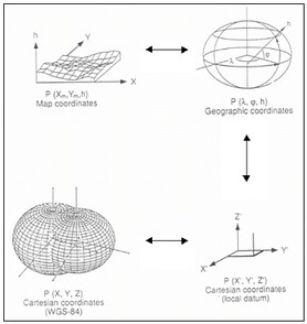
During the geocoding procedure, geodetic and cartographic transforms (refer to figure below) are considered in order to convert the geocoded image from the Global Cartesian coordinate system (WGS-84) into the local Cartographic Reference System (e.g. UTM-32, Gauss-Krueger, Oblique Mercator, etc.).

carto_system

In case of precise satellite orbits, the geocoding process is run in a fully automatic way. However, in case of inaccuracy in the satellite orbits, a Ground Control Point is required to precisely geolocate the input SAR data. As said above, the GCP is not needed if the manual or the automatic correction procedure has been previously executed.

Local Incidence Angle and Layover/Shadow

It represents the angle between the normal to the backscattering element and the incoming radiation.

Radiometric Calibration

Radars measure the ratio between the power of the transmitted pulse and the power of the received echoes. This ratio is called backscatter. The calibration of the backscatter values is necessary to compare radar data acquired with different sensors, in different acquisition modes, at different times, or generated by different processors.

The radiometric calibration of SAR data is carried out by following the radar equation law. It involves corrections for:

The scattering area (A) - Each output pixel is normalised for the real illuminated area of each resolution cell, which may change depending on topography and incidence angle. It is important to mention that this area can be: i) estimated considering the sine of the "local incidence angle"; ii) determined by computing the "true area".

The antenna gain pattern (G2) - The antenna gain variations in range are corrected taking into account the actual topography (Digital Elevation Model) or the reference ellipsoidal height. The antenna gain can be expressed as the ratio between the received signal and the transmitted signal or by comparing a real antenna to an isotropic antenna; it is measured in dB.

-	The range spread loss (R3) - The received power (backscattered signal) is corrected by taking into account the sensor-to-ground distance variation from the near range to the far range.

The formula applied for the radiometric calibration is (Holecz et al., 1993 and 1994):

new_radar_equation

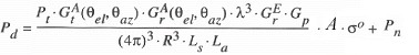
where Pd is the received power for distributed scatterers, Pt is the transmitted power, Pn is the additive power, G A is the transmitted and received antenna gain, G E is the electronic gain in radar receiver, Gp is the processor constant, R is the range spread loss, θel is the antenna elevation angle, θaz is the antenna azimuth angle, L are atmospheric (a) and system (s) losses, A is the scattering area.

In order to properly determine all required geometric parameters, which are used in the radar equation – and especially for the calculation of the local values – a Digital Elevation Model must be inputted; for this reason the calibration is performed during the data geocoding step, where the required parameters are already calculated.

The calibrated value is a normalized dimensionless number (linear units); the corresponding value in dB (10*log10 of the linear value) can be additionally generated by checking the relevant flag. The calibrated value can be generated as Sigma Nought, Gamma Nought and Beta Nought, by setting the appropriate flag in the Preferences>Geocoding (Backscatter Value section).

Radiometric Normalization

Even after a rigorous radiometric calibration, backscattering coefficient variations are clearly identifiable in range direction and in presence of topography. Note that these variations are an intrinsic property of each imaged object, and thus might be compensated, but it may not be corrected in absolute terms. The used method is named Cosine Correction:

•Cosine correction - a correction factor, which is based on a modified cosine model (Ulaby and Dobson, 1989), is applied to the backscattering coefficient to compensate for range variations according to:

•σοnorm = σοcal (cos ϑnorm / cos ϑinc )n

•

where n is a weighting factor, typically ranging from 2 to 7 depending upon the image acquisition mode (i.e the larger the incidence angle difference from the near to the far range, the higher n factor shall be set); ϑnorm is the incidence angle in the scene center (default setting); ϑin is the local incidence angle referred to the ellipsoid. The n factor can be set in the Preferences>Normalisation Factor. If a ϑnorm angle different from the scene center angle is required, it can be specified in the Preferences>Normalisation Angle.

Resampling

The peculiarity of the Optimal Resolution approach is that it allows avoiding the multi-looking step and it optimizes the resampling step (in geometric and radiometric terms). The four corner coordinates of each pixel in the Digital Elevation Model are independently projected (based on the range-Doppler equation) into the 1-look slant range geometry to form a polygon. The values of the pixels included within the polygon are subsequently added and the resulting averaged value, after the radiometric calibration and normalization, is assigned to the SAR geocoded output pixel. In this way, especially in hilly or mountainous terrain, the radiometry is preserved at the best. This approach should be used exclusively when single look data are geocoded to a significantly lower spatial resolution; in the other cases, the 4th Order Cubic Convolution method is recommended.

It is important to note that, if a Digital Elevation Model is used in input, it is automatically resampled to the output geocoding grid size using the 4th Order Cubic Convolution method.

Atmospheric Corrections

For some products, such as TerraSAR-X-1 and Tandem-X data, atmospheric related information are stored in one of the auxiliary files (i.e. "GEOREF.xml"). In this case, during the data import, the relevant factors are extracted from the "Signal Propagation Effects" section in order to be used for the correction of both the Scene Start Time and Slant Range Distance aimed at improving the product geolocation accuracy.

GCP file

In case a list of input files is entered, the data must be previously coregistered.

Meta file

This file is generated only when the "Input File List" contains more than 1 file and when the dimension of all the output files is the same. The meta file name prefix is the same as the first image in the input list.

Input Files

Input File List

Input file name(s) of all data to be geocoded. Intensity, amplitude as well as any other data type (coherence, interferogram, etc.) in slant or ground range geometry can be used. This file list is mandatory.

Optional Files

Geometry GCP File

Either a previously created Ground Control Point file (.xml) can be loaded (Select Geometry GCP File) or the interface to create a new Ground Control Point file is automatically loaded (Create GCP file, refer to the "Tools>Generate Ground Control Point" for details). This file is optional.

DEM/Cartographic System

DEM File

Digital Elevation Model (DEM) file name. This should be referred to the ellipsoid. In case a list of input files is entered, the DEM must cover the whole imaged area. This file is optional.

Output Projection

In case that the Digital Elevation Model is not used, it is mandatory to define the Cartographic System.

The Reset icon allows to reset the coordinate system field.

To use the same coordinate system as of another dataset, click the From Dataset button and select the source dataset.

To apply the same Coordinate System of the current selected layer, click the From Current View button.

Reference Height

In case that Digital Elevation Model is not used, a constant ellipsoidal height must be provided. The default reference height is 0.

Parameters - Principal Parameters

X Grid Size

The Easting (X) grid size of the output data must be defined; the default unit of measure is meters.

Note that for the Geographic projection, if values higher than 0.2 are entered they will be considered as metric units and then automatically, and roughly, converted from meters to degrees; if values lower than 0.2 are entered they will be considered as degree and used as such without any conversion.

Y Grid Size

The Northing (Y) grid size of the output data must be defined; the default unit of measure is meters.

Radiometric Calibration

By setting this parameter to True, radiometric calibration is performed.

Scattering Area Method

It can be determined using two different methods:

➢Local Incidence Angle - this is the fastest approach in terms of processing time, but it is not the most accurate way to calibrate the data in presence of topography.

➢True Area - it requires more computing resources, but it is the most accurate approach to calibrate the data in presence of topography. It makes sense to apply this method when a good (in terms of quality and spatial resolution) Digital Elevation Model is available.

Radiometric Normalization

By setting this flag radiometric normalization is performed.

Local Incidence Angle

By setting this flag the map of the local incidence angle – in degree – is generated.

Output type

By setting this flag the output type can be selected: calibrated products, dB units or both (default setting is linear units only).

Parameters - Global

It brings to the general section of the Preferences parameters. Any modified value will be used and stored for further processing sessions.

Parameters - Other Parameters

It brings to the general section of the Preferences parameters. Any modified value will be used and stored for further processing sessions.

Output Files

Output File List

Output file name(s) of all geocoded file(s). The number of output files must be equal to the number of input files. This file list is mandatory.

_geo

Geocoded Intensity/Power image and associated header files (.sml, .hdr). In case that radiometric calibration is selected, the output will contain geocoded backscattering coefficient values.

_geo_dB

Calibrated product in dB units and corresponding header file (.sml, .hdr). This file is generated only if the "Additional output dB" flag is selected.

_geo_lia

Geocoded Local Incidence Angle Map and corresponding header file (.sml, .hdr). This file is generated only if the "Local Incidence Angle" flag is selected.

_meta

It allows to load the geocoded outputs as a single file.

Please Note: the annotations of the geocoded files are displayed in ENVI View according to Preferences Common.

Details specific to the Units of Measure and Nomenclature of the output products can be found in the Data Format section.

General Functions

Store Batch

The processing step is stored in the batch list. The Batch Browser button allows to load the batch processing list.

Exec

The processing step is executed.

The window will be closed.

Help

Specific help document section.

Basic Module - Intensity Processing - Geocoding - Geocoding and Radiometric Calibration

Basic Module - Intensity Processing - Geocoding - Geocoding and Radiometric Calibration