Principal Component Analysis
Use PCA Rotation tools to perform principal component analysis (PCA; also called a PC transform) on multiband datasets. Data bands are often highly correlated because they occupy similar spectral regions. PCA is used to remove redundant spectral information from multiband datasets; thus it is one form of dimensionality reduction.
PCA is used in remote sensing to:
- Create a smaller dataset from multiple bands, while retaining as much original spectral information as possible. The result is a set of uncorrelated image bands, called PC bands.
- Reveal complex relationships among spectral features.
- Identify spectral characteristics that are more prevalent in most of the bands, and those that are specific to only a few bands.
PC bands will contain both data and noise. To separate noise from data, use the Minimum Noise Fraction (MNF) Transform tool instead.
In ENVI, you can run forward and inverse PC transforms. You can also compute and view statistics such as covariance, correlation, eigenvalues, and eigenvectors.
You can also write a script to perform principal components analysis using the ForwardPCATransform task.
See the following sections:
Background
PCA is a linear transformation that reorganizes the variance in a multiband image into a new set of image bands. These PC bands are uncorrelated linear combinations of the input bands. A PC transform finds a new set of orthogonal axes with their origin at the data mean, and it rotates them so the data variance is maximized. A more detailed discussion of PCA is available in most remote sensing literature.
ENVI performs the following steps to perform PCA:
- Compute the input image covariance or correlation matrix, depending on user preference.
- Compute the eigenvectors of the covariance or correlation matrix. See View PC Statistics below for more information on interpreting these statistics.
- Subtract the band mean from the input image data. This correction produces an origin shift in the output PC image such that its mean spectrum is 0 in every band.
- Project the mean-corrected image data onto the transpose of the eigenvector matrix, using the same approach as Richards (1999) but using the following equation:
y = G # (x-mean)
Where:
y = Transformed (or rotated) data
G = Transformation matrix
x = Input data
# Denotes matrix multiplication
An inverse PC rotation is computed by projecting the PC-rotated image data onto the inverse of the PCA transformation matrix.
You can calculate the same number of output PC bands as input bands. The first PC band contains the largest percentage of data variance, the second PC band contains the second largest data variance, and so on. The last PC bands appear noisy because they contain very little variance, much of which is from noise in the original spectral data. See Eigenvalues below for more information.
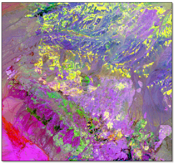
PC bands produce more colorful composite images than spectral color-composite images because the data is uncorrelated. Here is an example of a forward PC-rotated, color-composite image from Landsat-7:

Forward PC Rotation
You can perform a forward PC rotation based on new statistics, or from existing statistics.
Compute New Statistics and Rotate
Follow these steps to compute the eigenvalue and covariance or correlation statistics for your data and to perform a forward PC transform.
- From the Toolbox, select Transform > PCA Rotation > Forward PCA Rotation New Statistics & Rotate. The Principal Components Input File dialog appears.
- Select an input multiband file and perform optional spatial and spectral subsetting, and/or masking, then click OK. The Forward PC Parameters dialog appears.
- Are set to the same values as adjacent bands
- Are interpolated from nearby bands
- Are set to a constant value
- Contain zero variance or large outliers
- Click Stats Subset to calculate the statistics based on a spatial subset or the area under an ROI. The calculated statistics are applied to the entire file or to a spatial subset of the file.
- Enter the Stats X/Y Resize Factors less than 1 in the appropriate fields to sub-sample the data when calculating the statistics. This increases the speed of the statistics calculations. For example, using a resize factor of 0.1 will use every 10th pixel in the statistics calculations.
- In the Output Stats Filename [.sta] field, enter a filename for the noise statistics.
- Select whether to calculate the PCs based on the Covariance Matrix or Correlation Matrix using the toggle button. Typically:
- Use Covariance Matrix when calculating the principal components. This is the most common method to use with the majority of remote sensing datasets.
- Use Correlation Matrix when the data range differs greatly between bands and normalization is needed. This method normalizes the input bands to zero mean and unit variance. It equalizes the influence of each band, inflating the influence of bands with relatively small variance and reducing the influence of bands with high variance.
- If you selected a mask in Step 2, enter a value for the output results in the Output Mask Value field. ENVI applies the mask for the statistics calculation and the masked areas of the output dataset are set to the entered mask value.
- Select output to File or Memory.
- If you selected a mask in Step 2, the Zero Out Masked Values toggle button appears. Masked pixels are excluded when calculating statistics. The statistics results are then applied to all pixels in the image when applying the forward PC transform. The default value for this toggle button is Yes, which means that masked pixels will be assigned values of 0 in the PC output. Setting this option to No means that the masked pixels will run through the same forward PC transform as non-masked pixels.
- From the Output Data Type drop-down list, select the data type of the output file.
- To use a subset from eigenvalues, use the Select Subset from Eigenvalues toggle button to select Yes or No.
- If you chose No to selecting a subset from eigenvalues, select the Number of Output PC Bands. The default number of output bands is equal to the number of input bands.
- Click OK.
- Select the Number of Output PC Bands. PC Bands with large eigenvalues contain the largest amounts of data variance, while bands with lower eigenvalues contain less data information and more noise. Sometimes, it is best to output only those bands with large eigenvalues to save disk space.
- Click OK. ENVI performs the transform and adds the output to the Layer Manager. The output PC rotation contains only the number of bands that you selected. For example, if you chose 4 as the number of output bands, only the first four PC bands appear in your output file.
If you have any bad bands in your dataset, you should use spectral subsetting to exclude them from PC analysis. A singularity error can occur when a bad band becomes a near-perfect linear combination of other bands. This can happen when bad bands:
If you chose No to selecting a subset from eigenvalues, ENVI performs the transform and adds the output to the Layer Manager. The PC Eigenvalues plot window also appears.
If you chose Yes to selecting a subset from eigenvalues, the Select Number of Output Bands dialog appears after you click OK. Each band is listed with its corresponding eigenvalue and the cumulative percentage of data variance contained in each PC band. Do the following:
Rotate from Existing Statistics
If you already calculated covariance and eigenvalue statistics for your data, you can use them as input into the PC transform. You can use any statistics file in the PC rotation that contains covariance and eigen statistics for the same number of bands as your input data. (You may have already calculated these statistics using the Statistics Toolbox options or during a previous PC rotation session.)
Note: If you need to prevent certain pixels from being used when computing the statistics for the Principal Components Analysis rotation, first make a mask of the bad pixels, then use Basic Tools > Statistics to compute the covariance statistics on the masked image. You can then use this statistics file to do the principal components analysis.
- From the Toolbox, select Transform > PCA Rotation > Forward PCA Rotation Existing Statistics. The Principal Components Input File dialog appears.
- Select an input file and perform optional spatial subsetting, and/or masking, then click OK. The Enter Statistics Filename dialog appears with all of the existing statistics files in the current input data directory listed, using the default file extension
.sta. - Select the statistics file. The Forward PC Parameters dialog appears.
- Select whether to calculate the PCs based on the Covariance Matrix or Correlation Matrix using the toggle button. Typically:
- Use Covariance Matrix when calculating the principal components. This is the most common method to use with the majority of remote sensing datasets.
- Use Correlation Matrix when the data range differs greatly between bands and normalization is needed. This method normalizes the input bands to zero mean and unit variance. It equalizes the influence of each band, inflating the influence of bands with relatively small variance and reducing the influence of bands with high variance.
- Select output to File or Memory.
- From the Output Data Type drop-down list, select the data type of the output file.
- Select the number of output PC bands by using one of the following options:
- To select the number of output bands without examining the eigenvalues, select No from the Select Subset from Eigenvalues toggle button, then set the Number of Output PC Bands.
- To select the number of output MNF bands by examining the eigenvalues, use the following steps:
- Select Yes from the Select Subset from Eigenvalues toggle button.
- Click OK. ENVI calculates the statistics and the Select Output PC Bands dialog appears, with each band listed with its corresponding eigenvalue. Also listed is the cumulative percentage of data variance contained in each PC band for all bands.
- Set the Number of Output PC Bands. For the best results, and to save disk space, output only those bands with high eigenvalues. Images with eigenvalues close to 1 are mostly noise.
- Click OK. When ENVI finishes processing, the PC Eigenvalues plot window appears and the PC bands are added to the Layer Manager.
Inverse PC Rotation
Follow these steps to transform principal components images back into their original data space.
- From the Toolbox, select Transform > PCA Rotation > Inverse PCA Rotation. The Principal Components Input File dialog appears.
- Select an input file and perform optional spatial and spectral subsetting, then click OK. The Enter Statistics Filename dialog appears with all of the existing statistics files in the current input data directory listed. The statistics files appear with the default file extension
.sta. - Select the statistics file saved from the forward PC rotation. The statistics file must exist before you select the inverse PC rotation.
- Select either Covariance Matrix or Correlation Matrix by clicking the Calculate using toggle button.
- If you want to inverse the images back to their original data space, select the same calculate method that you used in the forward rotation.
- Select output to File or Memory.
- From the Output Data Type drop-down list, select the data type of the output file.
- Click OK. ENVI adds the resulting output to the Layer Manager.
View Statistics
If you chose to export a statistics file during forward PC rotation, you can view the resulting statistics, eigenvalues, and eigenvectors. Follow these steps:
- From the Toolbox, select Statistics > View Statistics File.
- Select the statistics file (
.sta) that you created, and click Open. - In the Statistics View dialog, click the Locate Stat drop-down list and select an option. These are described below.
Basic Stats
The Basic Stats section lists the minimum, maximum, mean, and standard deviation pixel value for each PC band. Here is an example:

Covariance
A covariance matrix is a square, symmetric matrix of size [number of input bands, number of input bands]. The diagonal elements are band variances, and the off-diagonals are band covariances. The covariance matrix is computed before PCA runs. Here is an example from a six-band image:

Correlation
A correlation matrix shows the statistical correlation of each input band to other input bands. It is computed before PCA runs. Here is an example from a six-band image:

Eigenvectors
An eigenvector matrix shows the statistical correlation between the PCs (dependent variables, or rows) and the input image bands (independent variables, or columns).
The eigenvectors themselves indicate the proportion that each input image band contributes to each PC band. This is referred to as weighting or factor loading. The weighting of each input band is computed by squaring the input band's eigenvector element. Thus, the total contribution of all of the input bands to any given PC band is the sum of the squares of the PC band's eigenvector elements.
There is one eigenvector for each PC band, and each eigenvector contains one element for each input band. For example, a PC rotation of a 128-band input image produces 128 PC bands and 128 corresponding eigenvectors that each have 128 elements. The first element of the eigenvector coresponds to input band 1, the second element to input band 2, and so forth.
The following is an eigenvector matrix where the columns represent six input spectral bands and the rows represent eigenvectors:

Eigenvalues
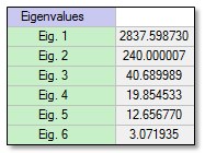
Eigenvalues indicate the length of each new PC, or the proportion of original information that each PC retains. From these values, you can derive the percentage of the total variance explained by each PC. To do this, compute the ratio of each eigenvalue to the sum of all of them. For example, the sum of all eigenvalues in the following table (for a six-band PC image) is 3153.8717:

The first component contains 89.97 % of the total variance: (2837.59873 / 3153.8717) * 100. The others are listed as follows:
|
Component |
% Total Variance |
Cumulative % |
|---|---|---|
|
PC Band 1 |
89.971906 |
89.971906 |
|
PC Band 2 |
7.6096945 |
97.581601 |
|
PC Band 3 |
1.2901599 |
98.871762 |
|
PC Band 4 |
0.6295288 |
99.501288 |
|
PC Band 5 |
0.401309 |
99.902594 |
|
PC Band 6 |
0.097402 |
100.0 |
From this table, you can see that the first three PC bands account for 98.87% of the total variance.
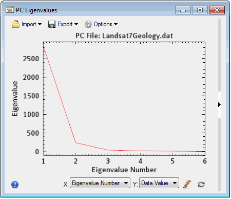
The PC Eigenvalues plot that is displayed after running a forward PC rotation shows a graphical representation of the relationship between eigenvalues (y-axis) and PC bands (x-axis):

Thus, eigenvalues are helpful in deciding which PCs will be of interest: typically those that retain the greatest amount of original information.
Chuvieco, E. Fundamentals of Satellite Remote Sensing: An Environmental Approach. 2nd ed. CRC Press, 2016.
Richards, J. A. Remote Sensing Digital Image Analysis: An Introduction, Springer-Verlag, 1999.