<< Click to Display Table of Contents >> Navigation:  Help Content > Interferometric Stacking > SBAS & E-SBAS > E-SBAS > Interferometric Stacking - SBAS & E-SBAS - E-SBAS Overview

A Note on the Enanched-SBAS functionality

 

The new E-SBAS technique identifies and process Permanent Scatterers pixels together with Distributed Scatterers ones. Providing a more comprehensive and valuable output. E-SBAS is capable of measuring Non-Linear displacement trend to both PS and DS pixels.

 

The proposed approach for E-SBAS is inspired by (Lanari, 2004). The deformation products will be obtained exploiting a combination of both Small Baseline subset (SBAS) and Persistent Scatterers Interferometry (PSI) methods, in order to estimate the temporal deformation at both DS and point-like PS. The low-pass (LP) and high-pass (HP) terms are used to name the low spatial resolution and residual high spatial frequency components of signals related to both deformation and topography.

 

The role of the SBAS technique is twofold: on the one hand, it will provide the LP deformation time series in correspondence of DS points and the LP DEM-residual topography; on the other hand, the SBAS will estimate the residual atmospheric phase delay still affecting the interferometric data after the preliminary correction carried out by leveraging GACOS products and ionospheric propagation models.

 

The temporal displacement associated to PS points will be obtained applying the PSI method to interferograms previously calibrated removing the LP topography, deformation and residual atmosphere estimated by the SBAS technique. This strategy “connects” the PSI and SBAS methods ensuring consistency of deformation results obtained at point-like and DS targets and, therefore, provides better results with respect to the approach of executing the two methods independently from each other.  The proposed hybrid approach is not just the simple application of the two techniques independently, indeed, the proposed approach is able to analyze both strong reflectors and distributed targets, delivering lower resolution DS results combined with higher resolution PS for even non-linear trends in an integrated continuous spatial solution.

 

The use of large temporal series enables to improve the identification and further removal of atmospheric related effects (artifacts) by means of a dedicated space-time filtering operation. A minimum number of three acquisitions is required to be able to run the processing, but more (at least twenty) are suggested to get reliable results especially in case of low coherence conditions.

 

The output products are stored in step-specific folders, which the program creates during the processing execution. These folders are automatically created inside the root output directory named using, as prefix, the "Output Root Name" and "_ESBAS_processing" as suffix, which is entered in the first processing step.

All intermediate files generated from each step are stored inside the _ESBAS_processing/work sub folder. In order to avoid processing failures it is recommended not to move any file from its original repository folder.

 

The "Auxiliary file" (marked by the name auxiliary.sml) is saved in the root output directory and it is updated during the execution of the different processing step. From the Interferometric Process step onwards, throughout the whole processing chain; it is important to note that the first input to enter, in any processing panel, is the "Auxiliary file". This file contains information to understand which steps have been executed, and what are the products generated.

The "work_parameters.sml" is saved in the work sub folder and contains information about the processing parameters setting.

 

It is possible to copy the whole [rootname]_ESBAS_processing folder together with the input and DEM files to another location/another drive (e.g. if the disk is full). The process can be resumed from the break point simply by re-launching the Connection Graph (inserting the inputs in the new location). Once the new Auxiliary file has been created it is necessary to edit it by inserting the DEM path in the new location and setting to "OK" or "NotOK" according to the steps performed in the previous location.

 

It is important to know that constant displacements, which affect all the area in the observed "Geographical Region", are not detected.

 

Notes:

•Please do not create your results in a folder containing spaces in the path.

•Once the output is created, the maximum number of files that can be opened is 130 due to the open capabilities files number of files opened in Windows (130x3 considering all the auxiliary files for single shape as .shp, .shx, .dbf). If the value exceeds 130, the process may slow down.

•

 

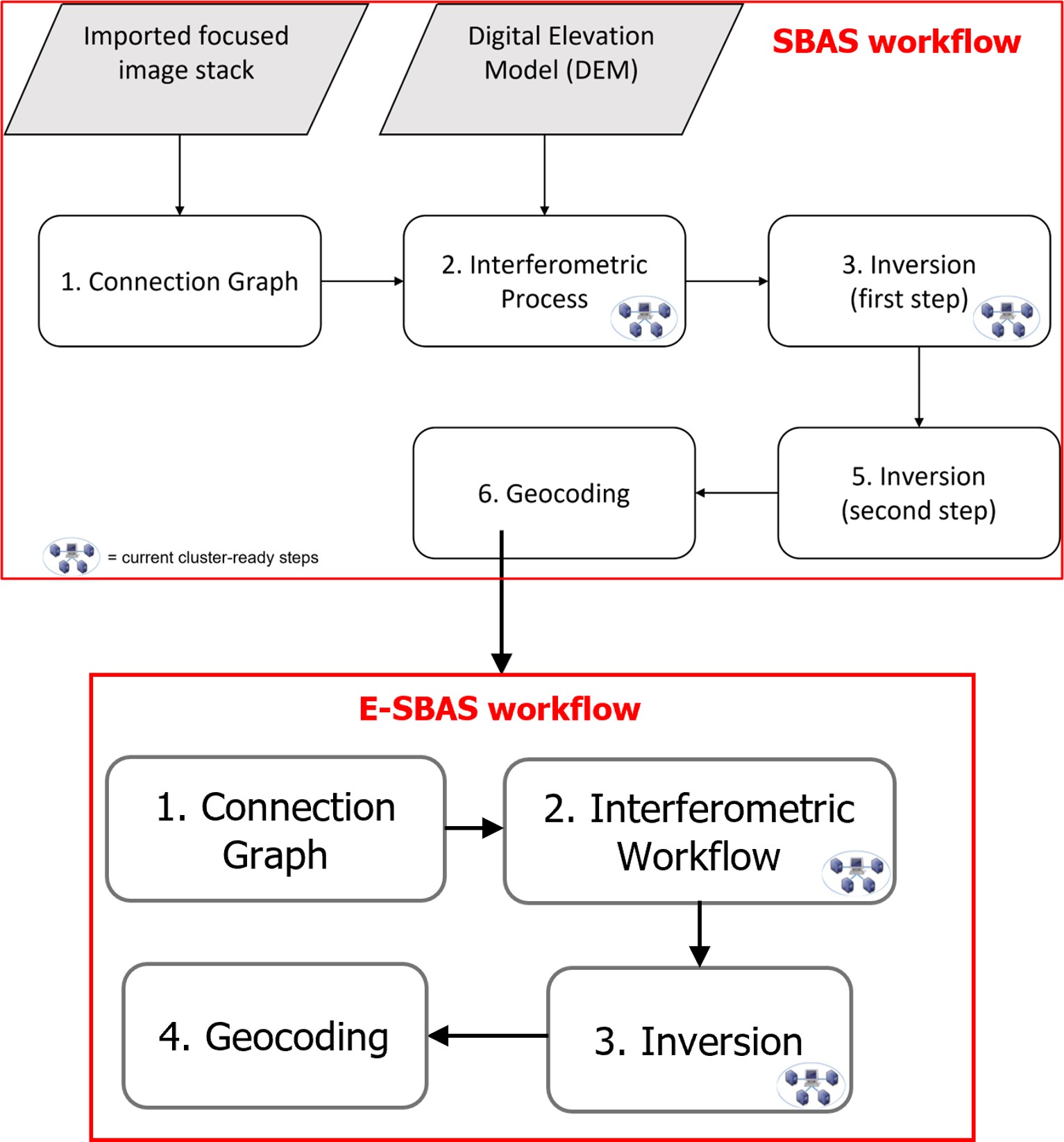
The processing sequence is depicted in the following block diagram. Please note that executing the SBAS processing chain is mandatory before proceeding with the E-SBAS workflow:

 

 

 

References

 

R. Lanari, O. Mora, M. Manunta, J. J. Mallorqui, P. Berardino and E. Sansosti, "A small-baseline approach for investigating deformations on full-resolution differential SAR interferograms," in IEEE Transactions on Geoscience and Remote Sensing, vol. 42, no. 7, pp. 1377-1386, July 2004.