Scatterplots
This topic presents two basic examples using the SCATTERPLOT function. The first plots impact crater data with a regression line and the second creates a plot of pixel values in two different bands of an image.
Scatterplot with Simple Regression Line
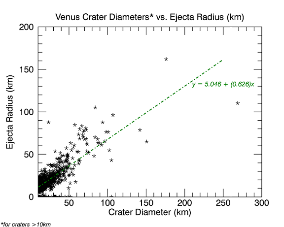
The \examples\data directory of your IDL installation contains a file named "VenusCraterData.csv", which, oddly enough, contains basic information about impact craters on Venus. We will use this data to construct a simple SCATTERPLOT and accompanying regression line using LINFIT and PLOT.
"VenusCraterData.csv" contains the following fields:
- Name: the official IAU name of the crater.
- Latitude : latitude of crater's center. Error is ±0.05°.
- Longitude: longitude of crater's center. Error is ±0.05°.
- Rim-to-Rim Diameter (d): mean diameter of the crater, in kilometers.
- dnd: difference in backscatter between a representative location on the crater floor (dni)and of a location in the terrain surrounding the crater (dno). One DN = 0.2 dB of RADAR backscatter.
- Ejecta Radius (erad): mean radius of the ejecta apron of the crater, in kilometers.
- Central Structure Diameter (Cd): diameter of a circle with an area equivalent to that encompassing any central structure, in kilometers.
To generate the plot above, copy and paste the following code at the IDL command line.
; Create the base template. Navigate to 'VenusCraterData.csv'
; in the \examples\data directory of your IDL installation.
; Fields are: Name, lat, long, diameter, dnd, erad, cstruct
myTemplate = ASCII_TEMPLATE()
; Read in the data. Make sure that \examples\data is in your IDL path.
craters = READ_ASCII('VenusCraterData.csv', TEMPLATE=myTemplate)
; Re-assign the crater variables to make them easier to type.
x = craters.diameter
y = craters.erad
;;----------------------------------------
;; This block is optional and uses an alternate read method.
;; Replaces the above lines of code.
;; Uncomment this block before copying/pasting
;; to the IDL command line.
;file = FILEPATH( "VenusCraterData.csv", $
; SUBDIRECTORY=['examples','data'] )
;craters = READ_CSV(file, COUNT=nRows, N_TABLE_HEADER=1)
;PRINT, nRows
;; Show information on the file structure
;HELP, craters, /STRUCTURES
;; Create aliases for the field names we want to use.
;x = craters.FIELD4 ;crater diameter
;y = craters.FIELD6 ;ejecta radius
;;----------------------------------------
; Now create the SCATTERPLOT, setting the XRANGE to mirror the
; actual range of the data in the file.
myPlot = SCATTERPLOT(x, y, SYMBOL='*', XRANGE=[10,300], $
TITLE='Venus Crater Diameters* vs. Ejecta Radius (km)', $
XTITLE='Crater Diameter (km)', $
SYM_SIZE=1.0, YTITLE='Ejecta Radius (km)')
; Calculate the values to fit into the regression line equation
; of y = A + Bx. Set up variables to hold the other values
; generated by LINFIT.
myLine = LINFIT(x, y, CHISQR=chisqr, COVAR=covar, $
MEASURE_ERRORS=measures, PROB=prob, SIGMA=sigma, $
YFIT=yfit)
; Plot the regression line by plugging the calculated A and B
; values into the equation y = A + Bx. See below.
; Use FINDGEN(250) to generate the x values to plug
; into the equation.
myX = FINDGEN(250)
myY = (5.046 + (0.626)*(myX))
myLineEq = PLOT(myX, myY, /OVERPLOT, COLOR='green', $
THICK=2, LINESTYLE=3, XRANGE=[10,300])
; Add some text to display the regression equation and a
; notation about the data included in the plot.
myText = TEXT(210, 130, 'y = 5.046 + (0.626)x', FONT_COLOR='green', $
FONT_SIZE=9, FONT_STYLE='italic', /DATA, TARGET=myPlot)
myText2=TEXT(1, 1, '*for craters >10km', FONT_COLOR='black', $
FONT_SIZE=8, FONT_STYLE='italic', /DEVICE, TARGET=myPlot)
; Display the A and B values of the regression line.
PRINT, myLine
IDL displays:
5.04582 0.626086
Notice that we did not use the other variables generated by the LINFIT function (such as CHISQR, etc.). You may optionally use TEXT to display them on your plot or use them in your paper or presentation.
Scatterplot of Image Data
You can create a SCATTERPLOT using two bands of image data. Two-dimensional (2D) scatterplots show the range of pixel values in each band, creating a visual way to assess data variance.
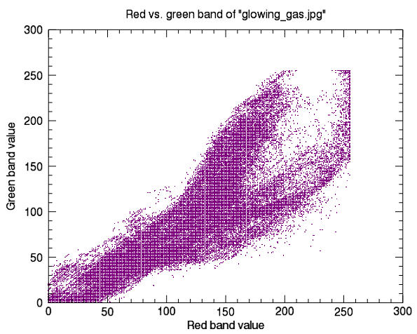
The code shown below creates the graphic shown above. Copy the entire block and paste it into the IDL command line to run it.
; Read in a 2-band image.
file = FILE_WHICH('glowing_gas.jpg')
!null = QUERY_IMAGE(file, info)
gas = READ_IMAGE(file)
red_band_pixels = REFORM(gas[0,*,*], PRODUCT(info.dimensions))
green_band_pixels = REFORM(gas[1,*,*], PRODUCT(info.dimensions))
; Plot red versus green band.
myPlot = SCATTERPLOT(red_band_pixels, green_band_pixels, $
SYMBOL = 'dot', /SYM_FILLED, SYM_COLOR = 'purple', $
XTITLE = 'Red band value', $
YTITLE = 'Green band value', $
TITLE = 'Red vs. green band of "glowing_gas.jpg"')
Resources and References
The version of the Venus Crater database in this example is excerpted from the one accompanying the chapter in the Venus II book entitled "Morphology and Morphometry of Impact Craters", by Robert R. Herrick, Virgil L. Sharpton, Michael C. Malin, Suzanne N. Lyons, and Kimberly Feely (1997, U. of Arizona Press, eds. S. W. Bougher, D. M. Hunten, and R. J. Phillips, pp. 1015-1046).
The original version of the database (release 1) was used for an article by Robert R. Herrick and Roger J. Phillips (1994, Implications of a global survey of Venusian impact craters, Icarus, v. 111, 387-416).