Filled Contours
You can enhance contour graphics by displaying different levels of the contour and filling them with color. In this topic, we will use the CONTOUR function along with various keywords to demonstrate some of the capabilities of CONTOUR.
For additional examples using CONTOUR, see the Environmental Monitoring Long Example.
Smoothed Contour Example
This first example uses random data to demonstrate how to define colors to use, fill the contours and then outline the levels you want to show. This example also illustrates how to smooth contour data.
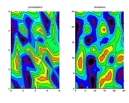
The code shown below creates the graphic shown above. You can copy the entire block and paste it into the IDL command line to run it.
; Create a simple dataset:
data = RANDOMU(seed, 9, 9)
; Plot the unsmoothed data:
unsmooth = CONTOUR(data, TITLE='Unsmoothed', $
LAYOUT=[2,1,1], RGB_TABLE=13, /FILL, N_LEVELS=10)
; Draw the outline of the 10 levels
outline1 = CONTOUR(data, N_LEVELS=10, /OVERPLOT)
; Plot the smoothed data:
smooth = CONTOUR(MIN_CURVE_SURF(data), TITLE='Smoothed', $
/CURRENT, LAYOUT=[2,1,2], RGB_TABLE=13, $
/FILL, N_LEVELS=10)
; Draw the outline of the 10 levels
outline2 = CONTOUR(MIN_CURVE_SURF(data), $
N_LEVELS=10, /OVERPLOT)
Digital Elevation Model (DEM) Contour Example
The data in this example is a digital elevation model (DEM) data taken from the Santa Monica mountains in California.
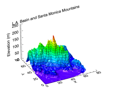
The code shown below creates the graphic shown above. You can copy the entire block and paste it into the IDL command line to run it. The keywords used are explained in detail after the example code.
; Define the digital elevation model data to open.
file = FILEPATH('elevbin.dat', SUBDIR=['examples', 'data'])
; Read the binary file and define the data dimensions.
dem = READ_BINARY(file, DATA_DIMS=[64,64])
; Rotate the data for display purposes.
dem = ROTATE(dem, 1)
; Define the minimum data elements.
dem_min = MIN(dem, MAX=dem_max)
; Define the number of levels to display.
nlevels = 15
; Define the levels to display.
levels = FINDGEN(nlevels)/nlevels*(dem_max-dem_min) + dem_min
; Define the levels to show and the colors to use.
levels = [-1, levels]
; Display the filled contour.
c1 = CONTOUR(dem, C_VALUE=levels, $
RGB_TABLE=34, /FILL, PLANAR=0, $
XTITLE='X', YTITLE='Y', ZTITLE='Elevation (m)', $
TITLE='L.A. Basin and Santa Monica Mountains')
; Move the Z Axis to the back by changing its location property.
(c1['zaxis']).location = [0, (c1.yrange)[1], 0]
; Overplot the contour lines to show more detail.
; Do not display the labels for the contour lines.
c2 = CONTOUR(dem, C_LABEL_SHOW=0, $
C_VALUE=levels, PLANAR=0, COLOR='black', $
/OVERPLOT)
Explanation of some of the properties and keywords used in the code above:
- In the first call to CONTOUR, C_VALUES sets the levels of the contours to the defined variable.
- The use of "/FILL" turns on the filling of the contour levels using the assigned color table. There are two ways to turn on FILL:
- /FILL
- FILL=1
- By default, CONTOUR sets the PLANAR property to one which turns on projecting the contour levels onto a 2-dimensional plane. When PLANAR is set to zero, it turns off this projection onto a 2-dimensional plane and allows the contours to occupy 3-dimensional space. It effectively turns the output from CONTOUR into a SURFACE plot.
- In the second call to CONTOUR, we turn off the labels by setting C_LABEL_SHOW to zero.
- In this call, not specifying the FILL property sets it to zero (the default) and allows just the contour lines to be drawn in 3-dimensional space (with PLANAR=0).