Texture Metrics Background
In general, texture refers to the spatial variation of image greyscale levels (tone) as a function of scale. When combined with spectral data, texture provides another level of information for interpreting features in pixel-based classification.
See the following sections:
- Process for Computing Texture Metrics
- First-Order (Occurrence) Metrics
- Second-Order (Co-occurrence) Metrics
Process for Computing Texture Metrics
A moving window, or kernel, is used to compute different texture metrics such as mean, variance, and entropy. Once you specify the size of the kernel (for example, 3 x 3 pixels), the process for computing texture metrics begins:
- If the DN values within the kernel are floating-point or double-precision, ENVI quantizes them into integer values.
- ENVI computes a histogram that determines the frequency of occurrence of the quantized values within the kernel.
- It creates a vector (1D array) of the occurrence values.
- It normalizes the occurrence values by dividing them by the number of values in the kernel (9 in this example). These are called probabilities,
 .
. - It computes the texture metric by summing the normalized occurrence values and applying the relevant equation.
- It assigns the resulting value to the center pixel in the kernel.
- The kernel moves one pixel over, and ENVI repeats the texture calculation.
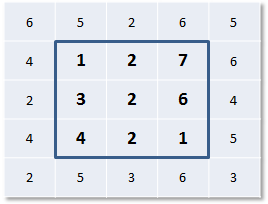

[0, 2, 3, 1, 1, 0, 1, 1]
[0.000, 0.222, 0.3.333, 0.111, 0.111, 0.000, 0.111, 0.111]
This process continues until every pixel in the image has a texture value.
The size of the kernel in part determines the success of texture-based image classification. If the window size is too small, you cannot extract enough spatial information to distinguish among different land features. If the window size is too large, it could overlap different features and introduce spatial errors (Anys et al., 1994).
Next are descriptions of the texture metrics that can be computed.
First-Order (Occurrence) Metrics
First-order metrics operate on the counts, or occurrences, of the different digital number (DN) values within a kernel. Separate images with different spatial arrangements of the same pixels within a single kernel will yield the same first-order texture value in both kernels.
For each pixel in the image, ENVI obtains the normalized histogram of its kernel and computes the first-order occurrence metrics below. The equations are from Anys (1994), where:
 = Probability of each pixel value
 = Number of distinct grey levels in the quantized image
You can compute the following first-order texture metrics:
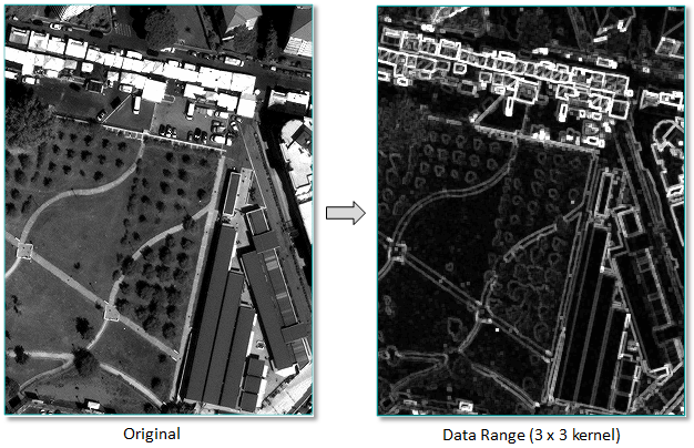
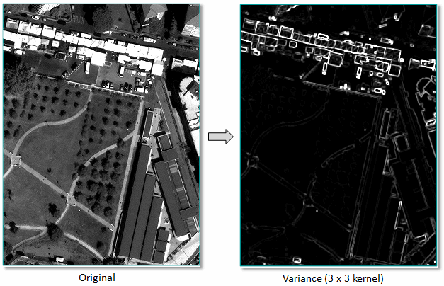
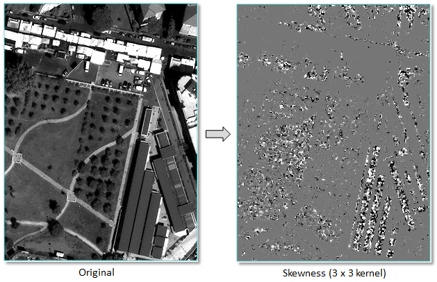
Along with the definitions of each texture measure below are images that show the results applied to WorldView-3 panchromatic scenes (40-centimeter resolution). The images are courtesy of DigitalGlobe. They provide examples of rough textures such as trees along with smooth, uniform textures such as building rooftops. Note how the results appear for various textures in these images.
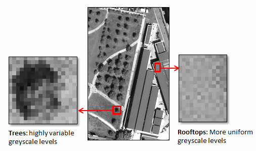
Data Range
This is the maximum value minus the minimum value in the kernel.
Mean
ENVI computes the mean of the kernel as follows. This is essentially a smoothing operation.


Variance
This is a measure of the dispersion of the values around the mean.

Entropy
ENVI uses the following equation from Anys et al. (1994) to compute entropy using the pixel values in a kernel centered at the current pixel. Entropy is calculated based on the distribution of the pixel values in the kernel. It measures the disorder of the kernel values.

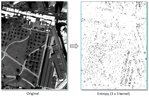
You can write a script to compute first-order entropy texture metrics using the ENVIFirstOrderEntropyTextureRaster routine.
Skewness
This is a measure of symmetry around the mean. The skewness for a normal distribution is 0. Negative values indicate data that are skewed left of the mean. Positive values indicate data that are skewed right.

Second-Order (Co-Occurrence) Metrics
Second-order (also called co-occurrence) metrics analyze the relationship between pixel pairs. They use a co-occurrence matrix to calculate texture values. This matrix is a function of both the angular relationship and distance between two neighboring pixels. It shows the number of occurrences of the relationship between a pixel and its specified neighbor. Haralick, Shanmugan, and Dinstein (1973) refer to this as a "gray-tone spatial-dependence matrix." Their implementation considers four directions (0°, 45°, 90°, and 135°) between neighboring cells that are separated by some distance, d.
ENVI uses a similar method to compute a co-occurrence matrix by considering that each pixel (except for those on the periphery of an image) has eight neighboring pixels. It can move in one of the following [x, y] increments:
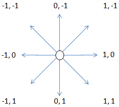
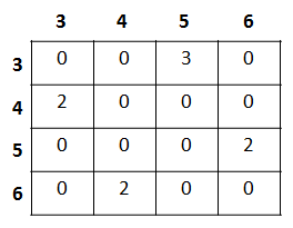
Assume that you have a 3 x 3 processing window over an image whose pixel values range from 2 to 6. Moving it one pixel to the right shifts it by 1 in the X direction and 0 in the Y direction as follows:

The co-occurrence matrix in this example would be as follows:
ENVI computes the following second-order co-occurrence metrics using the equations from Haralick, Shanmugan, and Dinstein (1973).
Mean
The local mean value of the kernel.

Variance
The local variance of the kernel. This value is based on the Greyscale Quantization Level that you specify.

The variable µ represents the mean of P.
Homogeneity
ENVI computes homogeneity using the "inverse difference moment" equation. Values range from 0 to 1.0.

Contrast
ENVI computes contrast using the following equation:

Dissimilarity
ENVI computes dissimilarity using the absolute values of the greyscale differences:

Entropy
Values range from 0 to the alog of the kernel size.

Second Moment
ENVI uses the "angular second moment" equation. Values range from 0 to 1.0.

Correlation
Values range from -1.0 to 1.0.

Anys, H., A. Bannari, D. C. He, and D. Morin. "Texture analysis for the mapping of urban areas using airborne MEIS-II images." Proceedings of the First International Airborne Remote Sensing Conference and Exhibition 3 (1994): 231-245.
Hall-Beyer, M. The GLCM tutorial home page. http://www.fp.ucalgary.ca/mhallbey/tutorial.htm. Updated February 2007. Accessed March 2016.
Haralick, R., Shanmugan, K., and Dinstein, I. "Textural Features for Image Classification." IEEE Transactions on Systems, Man, and Cybernetics 3, no. 6 (1973): 610-621.
Patel, D., and T. J. Stonham. "Texture Image Classification and Segmentation using RANK-Order Clustering." 11th IAPR International Conference on Pattern Recognition (1992), pp. 92-95.
Warner, T. "Kernel-based Texture in Remote Sensing Image Classification." Geography Compass 5/10 (2011): 781-798. doi: 10.1111/j.1749-8198.2011.00451.x
See Also
Texture Filters, Rank-Strength-Texture Algorithm Background, ENVIFirstOrderEntropyTextureRaster