Custom Plot Functions

This topic describes how to write custom ENVI plot functions in IDL. Plot functions provide a method for applying user-specified transforms to data in any ENVI plot window. You can choose a custom plot function from the Y: drop-down menu in any ENVI plot window.

Custom plot functions receive the input y values of an (x,y) plot and return the transformed y values to be plotted. Plot functions only operate on the y-axis data; the x-axis remains the same.

See the following sections:

• Write Custom Plot Functions
• Deploy Custom Plot Functions
• Example

Write Custom Plot Functions

The basic structure of a custom plot function looks like this:

FUNCTION My_Function_Name_custom_plot_function, $

  x, y, BBL_ARRAY=bblArray, _REF_EXTRA=refExtra

 

COMPILE_OPT idl2

 

  ; plot function here

 

END

Where:

• My_Function_Name_custom_plot_function: The name of the procedure. The function declaration must be appended with _custom_plot_function. Use an underscore when separating words in the function name.
• x: Input argument containing the X-axis values
• y: Input argument containing the Y-axis values
• BBL_ARRAY: Set this optional keyword to receive a byte array of ones and zeros representing which indices in the X and Y arrays are considered "good" and "bad." This typically would be used with a plot of a spectrum from a hyperspectral image. The number of elements of BBL_ARRAY will be the same as the X and Y arguments. This array is defined for all plots, regardless of the type of data. This keyword will only contain a value when a bad bands list is defined in the correponding ENVI header file.
• _REF_EXTRA: Set this required keyword to a variable that will collect all extra keywords that ENVI uses when calling the custom function.

The plot function can do anything to the incoming data array as long as the number of Y elements does not change. The X values are also sent in to the function and may be used if needed.

Save the code to a .pro file in IDL, or use the IDL SAVE command to create a .sav file.

Deploy Custom Plot Functions

Place the .pro file in the directory specified by the Custom Code Directory preference. The default location is as follows, where x_x is the ENVI version number:

Windows: C:\Users\username\.idl\envi\custom_codex_x

Linux: /home/username/.idl/envi/custom_codex_x

Example

This simple example plots the natural log (alog) of image data values. Follow these steps:

1. Start IDL and open a new IDL Editor window.
2. Copy and paste the following code into the IDL Editor:

FUNCTION Natural_Log_custom_plot_function, x, y, $

  _REF_EXTRA=refExtra

COMPILE_OPT idl2

 

 Return, Alog(y)

 

END

3. Save the program as Natural_Log_custom_plot_function.pro to your custom code directory, described above.
4. Start ENVI.
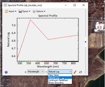
5. Open and display the file qb_boulder_msi from your default ENVI installation path.
6. Right-click anywhere in the image and select Profiles > Spectral. A Spectral Profile window appears.
7. From the Y: drop-down list, select Natural Log. The natural log plot is displayed; for example: