<< Click to Display Table of Contents >> Navigation:  Help Content > Interferometry Module > Displacement Modeling > Displacement Modeling - Graphic Viewer

 

 

Purpose

The graphic viewer is a simple interface with predefined settings to see datasets and sources, in 2D or 3D, allowing to save ready-to-use images in several formats.

 

Technical Note

The viewer can display 2D geocoded maps of InSAR and GPS datasets, 2D or 3D geocoded maps with one or more sources, 2D frontal view (i.e. in the strike/dip coordinate system) of elastic dislocation or opening sources. Graphic elements in the viewer can be arranged (resized, moved, rotated) to get the desired layout before saving it to PDF, TIFF or JPG, with a resolution compatible with scientific publications. Double clicking on graphic elements allows to access the IDL interface to set object properties. When the panel is resized, graphic elements are resized accordingly.

The graphic viewer behaves differently according to the context.

 

Input Dataset (Plot 2D)

 

 

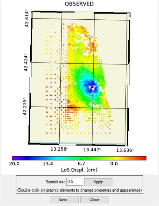
A simple maps with the observed points and a color bar is displayed, for InSAR data. Only the symbol size can be modified.

 

 

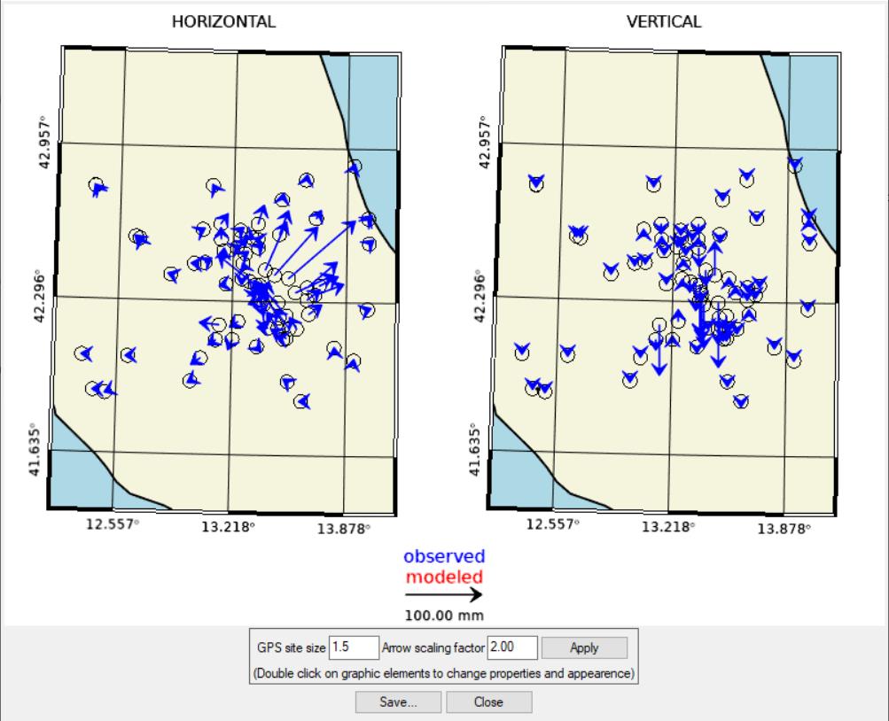
GPS observed data are shown with blue arrows in two different maps with horizontal and vertical components. Options are available to resize GPS site symbol and the arrow scale.

 

 

Output Dataset (plot 2D)

 

 

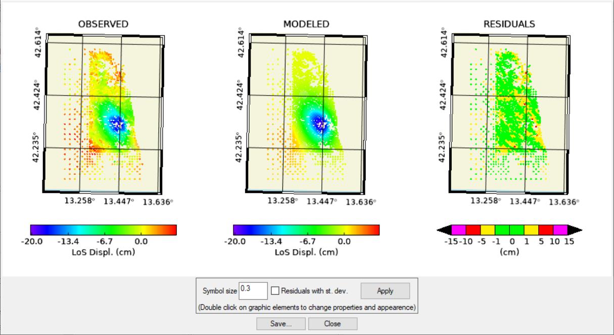
After Non-Linear and Linear inversion, InSAR datasets are shown in three maps: observed, modeled and residuals. Observed and modeled share the same color bar allowing a straight comparison. Residuals have a fixed color bar, in cm: intervals and colors are related to mean values for two-pass interferometry. Different intervals, problem dependent, can be obtained with “Residual with st. dev.” option (one sigma each interval)

 

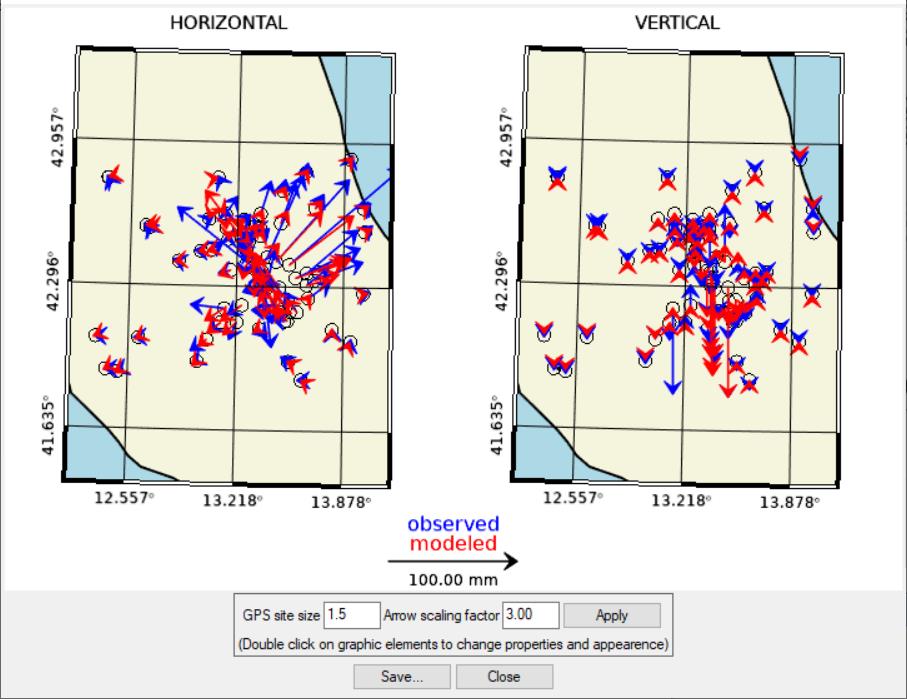
For GPS, observed arrows are overlapped to the modeled, in red, sharing the same scale.

 

Source plotting

The graphic viewer can display one or more sources simultaneously (if none is selected from the list, all are displayed). Slip, opening and CFF values are displayed with different color bars. If more sources with the same attribute (slip, opening or CFF) are present, the color bar for that attribute is unique. Sources without any attribute to show, as those in the Linear Inversion input, are plotted without colors.

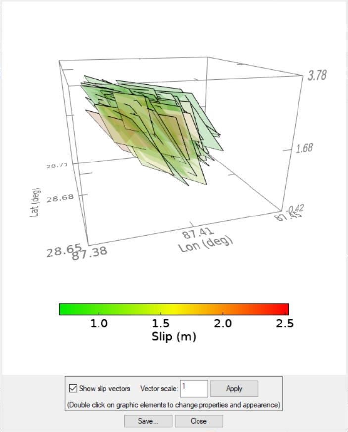
Three visualization type are implemented: 2D geocoded, 2D frontal (in strike/dip coordinates) and 3D geocoded.

 

Here some examples:

 

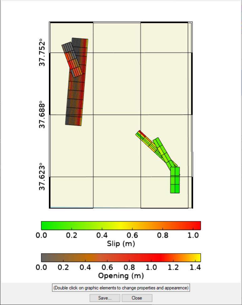
2D geocoded map with the result of a linear inversion, using three dislocation sources for an earthquake and two opening sources predicting a dike magma intrusion.

 

 

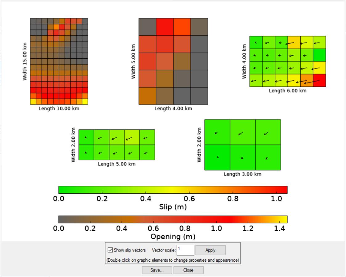
Same sources with 2D frontal view, i.e. strike/dip coordinates.

 

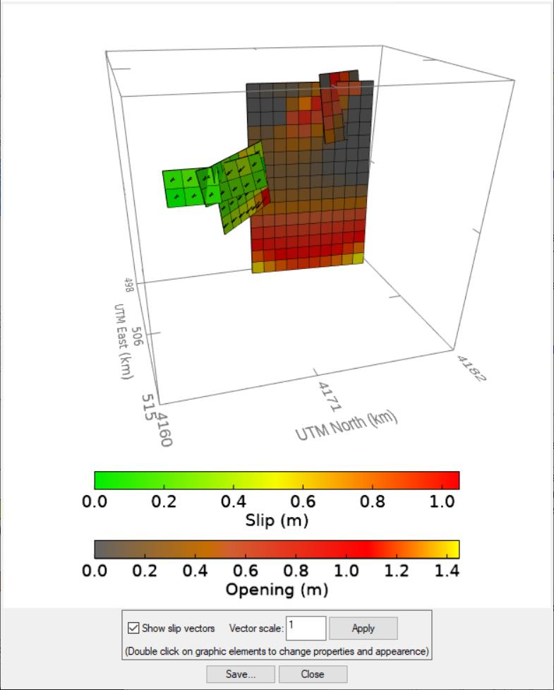
Same sources in a 3D geocoded view. Labels can be switched on/off with double click on the box axes, to keep them in foreground after rotating the data space.

 

 

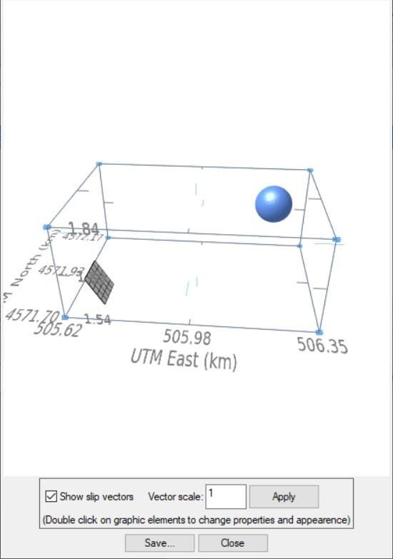
Dislocation source, without attributes, and a point pressure source; point pressure sources are sized according to the volume variation.

 

Another useful use of the graphic viewer is to inspect the results of the statistical analysis, in the on-Linear inversion (‘OUTPUT Statistics’ folder): it is possible to see the cloud of solutions corresponding to the inversion of datasets perturbed with ad hoc noise. A quantitative assessment (uncertainty and trade-offs) is also available in the ‘VIEW SOURCES – Plot Statistics’ menu.

 

Specific functions

Different options are available according to the context the viewer is invoked. In the above examples all the possible options.

 

General function

 

SAVE… : allow to save the viewer content to PDF, TIFF or JPG format

CLOSE: close the panel