<< Click to Display Table of Contents >> Navigation:  »No topics above this level« Basic - Intensity Processing - Filtering - Multi-temporal ANLD filtering

Purpose

 

Images obtained from coherent sensors such as SAR (or Laser) system are characterized by speckle, This is a spatially random multiplicative noise due to coherent superposition of multiple backscatter sources within a SAR resolution element. In other words, speckle is a statistical fluctuation associated with the radar reflectivity of each pixel a scene. A first step to reduce the speckle - at the expense of  spatial resolution - is usually performed during the multi-looking, where range and/or azimuth resolution cells are averaged.

 

Whenever two or more images of the same scene taken at different times are available, multi-temporal speckle filtering – which exploits the space-varying temporal correlation of speckle between the images – should be applied, in order to reduce this system inherent multiplicative noise.

 

Technical Note

 

Multi-temporal Anisotropic Non-Linear Diffusion Filter

Single-date and multi-temporal SAR filtering methods, based on probability density functions, perform well under strictly controlled conditions, but they are often limited with respect to sensor synergy – where complex joint probability density functions must be considered – and to the temporal aspect. The drawback of existing multi-temporal speckle filters is that they are strongly sensor and acquisition mode dependant, because based on statistical scene descriptors. Moreover, if features masks are used, an accuracy loss can be introduced when regarding particular shape preservation, mainly due to the lack of a priori information about size and type of the features existent in the image. Therefore, in order to take advantage of the redundant information available when using multi-temporal images acquired with different geometries, while being fully independent regarding the data source, a hybrid multi-temporal anisotropic diffusion scheme can be applied. In this case, the multi-temporal SAR data set must be either geocoded (different acquisition geometries case) or co-registered (same SAR sensor with the same acquisition geometry).

 

In case of geocoded data, the grid size must be the same for all the images in the multi-temporal series.

 

With respect to the approach described for the Single Image>Anisotropic Non-Linear Diffusion filters, in the multi-temporal case the choice is made to measure the gradient using the whole set of images. The most natural choice is then to use the reliable formulation for gradient computation with vector data, which takes the gradient as two dimensional manifold embedded in ℜm, obtaining the following First Fundamental Form (FFF):

 

 

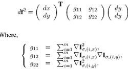
where Iσ2(i,x) and Iσ2(i,y) stands respectively for gradient estimation along columns and lines. The direction and magnitude of the maximum and minimum rate of change corresponding to the computed gradient directions can be then extracted from the FFF eigenvalues and eigenvectors. Finally, the practical framework of the anisotropic diffusion process can be written as:

 

 

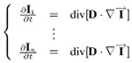
where I corresponds to the whole multi-temporal image sequence and Ii is the ith image in the sequence. Therefore, each image is filtered separately using the global sequence information, taking into account features from all images.

 

 

Please note:

Only calibrated data have to be used as input.

 

 

 

Input Files

 

Input file list

Input file names of coregistered (_pwr, _rsp) or geocoded (_geo) data. This file list is mandatory.

 

Parameters - Principal Parameters

 

In order to optimally exploit the potential of the Anisotropic Non-Linear Diffusion filter, the eight parameters listed here below shall be set/tuned depending on the input data. For instance different setting has to be considered when different data types (e.g. SAR amplitude, SAR Interferometric coherence, Optical images, etc.) or data with different spatial resolution are used as input.        

 

Gaussian Blur Kernel Variance

This parameter describes the size and amount of Gaussian applied to the image before performing the diffusion. Increasing the size of the kernel will lead to strongly smoothed image but also to the loss of image small details.

 

Window Size

The algorithm performs an adaptive threshold selection across the image in order to retrieve the adequate gradient values for preserving the edges. This is done by dividing the image in square windows where an individual threshold value is computed. Small windows will better keep fine details, while big windows will smooth more preserving only the most evident structures.

 

Anisotropy

This value can vary from 0 to 1. It tunes the amount of filter diffusion along the edges. Higher values increase the filtered edges sharpness, but possibly introduce edge deformations. Changing this parameter has an effect only whether some Anisotropic iterations are specified.

 

Step Size

This parameter is a positive integer that can be used to reshape the gradient sensitivity function of the diffusion. Low values of this parameters produce smooth curves (isotropic diffusion decreases slowly around edges) whereas high values lead to sharper curves (isotropic diffusion decreases quickly around edges).

 

Global Iterations

It determines the number of processing iterations (both non-linear and anisotropic diffusion steps).

 

Non-Linear Iterations

It determines the number of non-linear diffusion iterations. This part of the algorithm leaves the high gradient zones unfiltered. Therefore, it preserves the maximum of details while smoothing homogenous areas. It must be noted that, to have an evident effect in terms of filtering variation, the iterations number has to be modified with steps of 10.

 

Anisotropic Iterations

It determines the number of nonlinear diffusion iterations. This part of the algorithm smoothes the high gradient zones, improving the image edge appearance. It must be noted that, to have an evident effect in terms of filtering variation, the iterations number has to be modified with steps of 10.

 

Threshold Recomputation

Among the algorithm steps, the most time consuming is certainly the threshold estimation. This parameter adds the possibility to recompute the threshold for the number of iterations specified by the user. Setting it to values higher than 1 can considerably decrease the image processing time (especially when inputting large images) since the threshold are recomputed less times.

 

Parameters - Global

 

It brings to the general section of the Preferences parameters. Any modified value will be used and stored for further processing sessions.

 

Parameters - Other Parameters

 

It brings to the general section of the Preferences parameters. Any modified value will be used and stored for further processing sessions.

 

Output Files

 

Output file list

Output file list of the filtered data. This file list is mandatory.

 

_fil        

Filtered Intensity image and associated header files (.sml, .hdr).

 

_meta        

It allows to load the processing results as a single file.

 

Details specific to the Units of Measure and Nomenclature of the output products can be found in the Data Format section.

 

General Functions

 

Exec

The processing step is executed.

 

Store Batch        

The processing step is stored in the batch list. The Batch Browser button allows to load the batch processing list.

 

Close        

The window will be closed.

 

Help

Specific help document section.

 

 

Specific Function(s)

 

Anisotropic Non-Linear Diffusion        

 

-Commit

The new input parameters are stored.        

 

-Restore

The default parameter setting is reloaded.        

 

-Cancel

The window will be closed.

 

References

 

Aspert F., M. Bach Cuadra, J.P. Thiran, A. Cantone, and F. Holecz, Time-varying segmentation for mapping of land cover changes, Proceeding of ESA Symposium, Montreux, 2007.